Poisson Processes and Queues

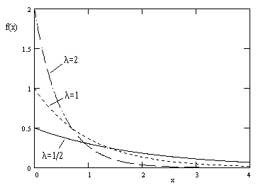
The occurrences of a sequence of discrete events can often be realistically modeled as a Poisson process. The defining characteristic of such a process is that the time intervals between successive events are exponentially distributed. Given a sequence of discrete events occurring at times t₀, t₁, t₂, t₃,..., the intervals between successive events are Δt₁ = (t₁ – t₀), Δt₂ = (t₂ – t₁), Δt₃ = (t₃ – t₂), ..., and so on. For a Poisson process, these intervals are treated as independent random variables drawn from an exponentially distributed population, i.e., a population with the density function f(x) = λe^-λx for some fixed constant λ. This distribution function is illustrated below for various values of λ.

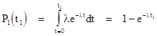
The exponential distribution is particularly convenient for mathematical modeling, because it implies a fixed rate of occurrence. To see why this is the case, suppose a system begins in State 0 at the initial time t = 0, and it will change to State 1 at the time t = T, where T is to be randomly drawn from an exponential distribution. What is the probability that the system will be in State 1 at some arbitrary time t₁? Clearly the answer is the integral of the probability density function from t = 0 to t = t₁. Letting P_j(t) denote the probability of being in State j at time t, we have

The probability of the system still being in State 0 at time t₁ is just the complement of this, i.e., we have P₀(t₁) = . Also, at any time t, the above equation shows that the absolute rate of change of the probability of being in State 1 is dP₁/dt = λe^-λt , so we have the useful relation

                                 (1)

Of course, since P₀ + P₁ = 1, we could replace P₀ with 1 – P₁ and write this as

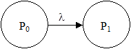
which is just a simple first-order lag with the "time constant" 1/λ, and the solution of this differential equation is just the expression for P₁ given above. The significance of equation (1) is that we can express the derivative of a state probability due to an exponential transition as the product of the transition rate λ and the probability of the source state. A single exponential transition with rate λ from one state to another can be represented schematically as follows:

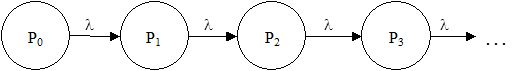
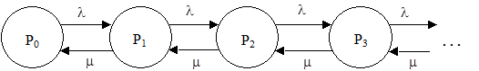
More generally, for any number of possible states, if the transitions from one state to another are all exponential, we can immediately write down the system of differential equations governing the probabilities of being in each of the states. This enables us to evaluate the behavior of a Poisson process, because (by definition) the transition time from the state P_n to the state of P_n+1 is exponential for all n. It's convenient to represent a simple Poisson process schematically as shown below.

Here P_j denotes the probability of the jth state, which is the state when exactly j events have occurred. These probabilities are functions of time, and we typically begin with the initial conditions P₀(0) = 1, P_j(0) = 0 for all j > 0. Given that the intervals between occurrences are drawn from an exponential distribution, we would like to know the probability that exactly n events have occurred by the time t. In other words, we want to determine the probability P_n(t).

Since all the transitions are exponentially distributed, we immediately have the equations

With the initial condition P₀(0) = 1, the first equation can be solved immediately to give P₀(t) = e^-λt. Substituting this into the second equation, we have

Recall that the general solution of any equation of the form dx/dt + F(t)x = G(t) is

where C is a constant of integration. Setting x = P₁, F(t) = λ, and G(t) = λe^-λt, we get r = λt and therefore

where we have set C = 0 to match the initial condition P₁(0) = 0. Substituting the expression for P₁(t) into the next system equation gives

which we can solve to give

where again we have set the constant of integration C to zero to match the initial condition P₂(0) = 0. Continuing in this way, it's easy to see by induction that the probability of the nth state at time t is

This is the probability distribution for a simple Poisson "counting" process, representing the probability that exactly n events will have occurred by the time t. Obviously the sum of these probabilities for n = 1 to ∞ equals 1, because the exponential e^–λt factors out of the sum, and the sum of the remaining factors is just the power series expansion of e^λt.

It's worth noting that since the distribution of intervals between successive occurrences is exponential, the Poisson distribution is stationary, meaning that any time can be taken as the initial time t = 0, which implies that the probability of n occurrences in an interval of time depends only on the length of the interval, not on when the interval occurs.

The expected number of occurrences by the time t is given by the integral

where we have again made use of the fact that the right hand summation is just the power series expansion of e^λt. (We also changed the lower summation bound from n = 0 to n = 1 because n appears as a factor of the argument, which makes the n = 0 term vanish.)

One typical application of exponential transitions and Poisson models is in the theory of queues. For example, suppose customers enter a shop at random times with a constant rate λ, and their orders are processed at a constant rate μ. How many customers will be waiting at any given time? We can model this process using exponential transitions as shown schematically below.

The nth state represents the state when n customers are waiting, and P_n(t) denotes the probability of that state at the time t. Each "λ transition" causes the system to change from the state n to the state n+1, and "μ transition" causes the state to change from the state n to the state n–1. At the beginning of the day, the shop is empty, i.e., the system is in the state 0 with probability P₀(0) = 1. The system dynamic equations can be written down immediately

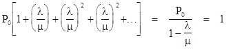
and so on. Often we are just interested in the steady-state probabilities, i.e., the distribution of probabilities once the system has reached equilibrium and has stabilized. This condition is characterized by the vanishing of all the derivatives of the probabilities, so the first equation implies P₁ = (λ/μ)P₀, and we can substitute this into the second equation to give P₂ = (λ/μ)²P₀, and so on. In general we have P_n = (λ/μ)ⁿP₀. Also, since the sum of all the probabilities equals 1, we have the geometric series

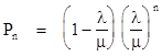
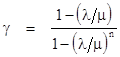
from which it follows that P₀ = 1 – (λ/μ) and therefore

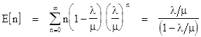
For our example of customers waiting in a shop, this gives the probability that exactly n customers are presently waiting (including those presently being served). The expected number of customers presently waiting (i.e., the mean length of the queue) is given by

This type of queue is sometimes designated as an M/M/1 queue, where the first M signifies that the arrivals are memoryless (i.e., exponentially distributed), the second M signifies the same for the departures, and the 1 signifies a single server. Naturally these system equations converge only if λ is less than μ (i.e., the rate of customer arrivals is less than the rate at which they are processed), since otherwise the queue will grow indefinitely.

It's also interesting to consider the actual time-dependent solution of the model. We can begin by examining a truncated version with just the two lowest states with probabilities P₀(t) and P₁(t). The system equations are

along with the condition P₀ + P₁ = 1. Substituting from this identity into the first system equation gives

With the initial condition P₀(0) = 1 the solution is

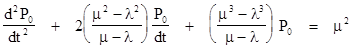
Similarly we can consider a finite system consisting of the three lowest states, which leads to the differential equation for P₀(t)

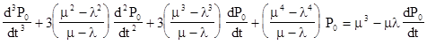
From this and the previous case we might be tempted to assume a general "binomial" form, but the simple pattern breaks down when we consider the system consisting of the four lowest states, leading to the differential equation

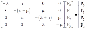
As more states are included, more "non-binomial" terms appear. However, there is a relatively simple pattern underlying this sequence of differential equations. To see this, consider the basic first-order system equations for the four-state system expressed in matrix form as shown below.

In general we can solve this eigenvalue problem by finding the roots of the characteristic polynomial, and for the n-state system we find n distinct roots, one of which is zero, corresponding to a constant of integration in the general solution of the differential. The other n-1 roots for the first several values of n are tabulated below:

Clearly the eigenvalues for the n-state system are

along with the eigenvalue 0. Notice that for even values of n the eigenvalue with k = n/2 is simply –(λ+μ). More generally, if n divides m, then the eigenvalues of the n-state system are a subset of those of the m-state system. Based on these eigenvalues, we know the general solution for the n-state system is of the form

where γ and the a_k and b_k are constants of integration, determined by the initial conditions. From the steady-state solution for the n-state system we have

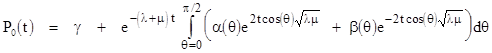
If we now consider the infinite-state system, the summation becomes an integration, the argument kπ/n becomes a real variable θ ranging from 0 to π/2, and the coefficients becomes continuous functions of θ. Thus we have

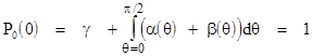
with the condition that

It's easy to verify convergence because the magnitude of the negative exponent –(λ+μ)t is always greater than or equal to the magnitude of the exponent 2t cos(θ) because with cos(θ) equal to its maximum value of 1 we can square both quantities and find the inequality (λ+μ)² ≥ 4λμ, which is equivalent to (λ-μ)² ≥ 0.

The above equation shows that the time-dependent probabilities in a simple M/M/1 queue are closely analogous to the coefficients of the Fourier series for the functions α(θ) and β(θ).

Return to MathPages Main Menu