The Gambler's Ruin

You always said the cards would never do you wrong;

The trick you said was never play the game too long.

                                                                      Bob Seger

Consider a game that gives a probability α of winning 1 dollar and a probability β = 1–α of losing 1 dollar. If a player begins with (say) 10 dollars, and intends to play the game repeatedly until he either goes broke or increases his holdings to N dollars, what is his probability of reaching his desired goal before going broke? This is commonly known as the Gambler's Ruin problem. For any given amount h of current holdings, the conditional probability of reaching N dollars before going broke is independent of how we acquired the h dollars, so there is a unique probability Pr{N|h} of reaching N on the condition that we currently hold h dollars. Of course, for any finite N we can immediately set  Pr{N|0} = 0  and  Pr{N|N} = 1. The problem is to determine the values of Pr{N|h} for h between 0 and N.

Suppose the player’s current holdings are h dollars, with a probability of Pr{N|h} of “winning”. The next round will leave him with either h+1 or h–1 dollars, and the probabilities of these two outcomes are α and 1–α respectively. Therefore, another way of expressing his current probability of winning is as a weighted average of the probabilities of winning in his two possible “next” states. Thus we have

This gives us a second-order linear recurrence relation that must be satisfied by the values of Pr{N|h}. The characteristic polynomial of this recurrence is

which has the roots 1 and r = (1–α)/α.  If these two roots are distinct (meaning that α is not equal to exactly 1/2), the general form of the recurrence solution is a linear combination of successive powers of these two characteristic roots. Therefore, the general solution of the recurrence is

where A and B are constants to be determined by our two boundary conditions, Pr{N|0} = 0 and  Pr{N|N} = 1.  Inserting these values gives the conditions

from which it follows that

Therefore, if a player is currently holding h dollars, his probability of reaching N dollars before going broke is

This was based on the assumption that α does not exactly equal 1–α, so r is not equal to 1.  If, on the other hand, α = 1/2, we see that our two particular solutions 1^h and r^h are not independent. In this case the characteristic polynomial has duplicate roots, but another independent solution of the recurrence (1) is given by Pr{N|h} = h.  Therefore, the general form of the solution is A + Bh, and our boundary conditions require A = 0 and B = 1/N, so the total solution in this special symmetrical case is

Hence, if we begin with 10 dollars, we have a 50% chance of reaching 20 dollars before going broke. Obviously we can replace 20 with any other threshold we choose. For any given initial holdings, if we increase our upper target from 20 to some larger number, we see that our probability of going broke before reaching that number also increases. If we have no "quit while we're ahead" target, and simply intend to play the game indefinitely, our probability of eventually going broke approaches 1, which presumably is why this problem is called the gambler's ruin. 

We can also consider the number of rounds that the player can expect to play before either going broke or reaching his goal. By reasoning analogous to what we used for the probabilities, we know that the expected number of rounds from a current holding of h dollars equals 1 plus the weighted average of the expectations for the two possible successor holdings, h+1 or h–1. In other words, the function giving the expected number or rounds satisfies the recurrence

This has the same homogeneous solution as the probabilities, but we must also determine a particular solution to be compatible with the inhomogeneous nature of the recurrence. To do this, notice that in terms of the successive differences D_n = E_n – E_n–1 we can re-write the equation in the form

The solution of this linear fractional recurrence is

Therefore we have the particular solution

Thus the particular solution is of the form E_n = C₁ + C₂ rⁿ + [(r+1)/(r–1)]n for constants C₁ and C₂, and we recall that the homogeneous solution is of the form A + Brⁿ for arbitrary constants A and B. The sum of the particular and homogeneous solution therefore is of the form

Imposing the boundary conditions E₀ = E_N = 0, we can determine the values of A and B, and this leads to the result

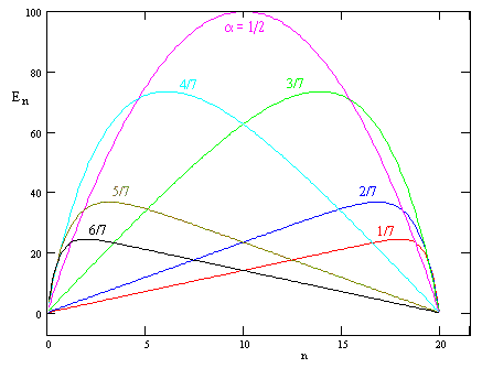
A plot of this function for N = 20 and various values of α = 1/(1+r) is shown below.

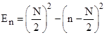
In the degenerate case with a = 1/2 the expected number of rounds beginning with n dollars is just the parabola

In the above discussion we considered only the case when each step changed our holdings by one unit, up or down. We can also treat the more general problem of allowing more than two possible outcomes of each round, and allowing the steps to be of arbitrary sizes. For example, we might consider a game that has three possible outcomes (on each round), with probabilities α, β, and γ changing our holdings by the amounts 2, +1, and –1 respectively. In this case the same reasoning that led to equation (1) leads to a third-order recurrence

In this case we have three boundary conditions  Pr{N|0} = 0,  Pr{N|N} = 1, and  Pr{N|N+1} = 1, noting that it's possible to end on either N or N+1. In this more general case we can proceed as before, by finding the roots of the characteristic polynomial, and then expressing Pr{N|h} as a linear combination of the hth powers of those roots, subject to the boundary conditions. This problem can be regarded as a one-dimensional random walk. 

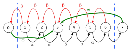
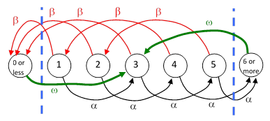
Another approach is to represent the game by a Markov model, and recursively generate the probabilities of having each particular value of holdings after the nth round of play, beginning from some specified initial holdings. This can be treated as a diffusion process, with absorbing states at all values less than 0 and greater than N, where all the probability eventually accumulates. However, it this game can also be solved by considering the steady-state transition rates of a closed-loop Markov model. To illustrate, consider again the original gambler’s ruin game, with the player’s holding increasing or decreasing by one dollar on each round with probability α and β = 1 – α respectively. For convenience, let the player’s target be 7 dollars and suppose he begins with 3 dollars. We can represent continual repetitions of this game by the model shown below.

The states labeled 0 and 7 are just formal, with zero probability, because we will set the feedback transition rate ω to infinity. At steady state we have the feedback flow rates

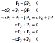
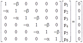
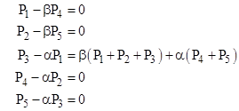
but we needn’t make use of these directly. From state 3, the probability of reaching state 7 before reaching state 0 is Pr{7|3} = αP₆/(βP₁ + αP₆). Note that P_j signifies the probability of the jth state, not the probability of winning from the jth state. The remaining steady-state system equations are

Since we care only about the ratios of the probabilities, we can re-normalize such that (αP₆ + βP₁) = 1, and then write the system equations in matrix form as

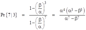
where we have used lower case p to denote the re-normalized probabilities. Solving this system of equations and inserting the resulting values of p₁ and p₆ into the expression  αp₆/(βp₁ + αp₆) gives the probability of reaching 7 (before reaching 0) from state 3 as

It may not be immediately apparent that this is consistent with our previous result, which was

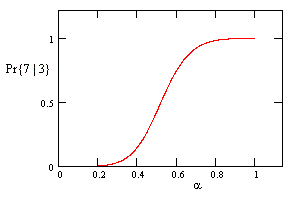
However, if we make the substitution β = 1 – α, both of these expressions give

This function is plotted in the figure below.

The same approach can be applied to more general cases. Suppose on each round a player has probability α of gaining 2 dollars and probability β = 1 – α of losing 3 dollars. Beginning with a specified number of dollars in the range from 1 to 5, what is the probability of reaching 6 or more prior to falling to 0 or below? For a player beginning with 3 dollars, we construct a closed-loop Markov model as shown below.

Again, the states labeled “0 or less” and “6 or more” are just formal, with zero probability, because we will set the transition rate ω to infinity. At steady state we have the “feedback flow rates

but we needn’t make use of these. The remaining steady-state system equations are

The four homogeneous equations give

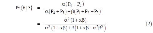
The rates of entering the two limiting states are α(P₄ + P₅) and β(P₁ + P₂ + P₃), so the probability of reaching 6 (or more) prior to falling to 0 or below, beginning from 3, is

Making the substitution β = 1 – α, we can express this purely as a function of α as follows:

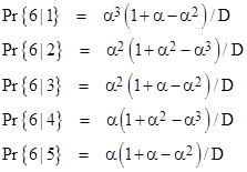
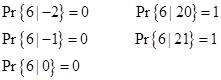
By re-directing the restoration paths from State 3 to one of the other states, we get the probabilities of “winning” beginning from each of the states. The results are summarized below.

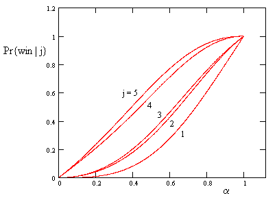
A plot of these five function is shown below.

The probability of winning with a beginning amount of 2 is nearly the same as with a beginning amount of 3.  Each of these has a probability β of losing on the first round, and even if they win on the first round, the jump to 4 and 5 respectively, which are also quite close, because they each have a probability α of winning on that round.

Incidentally, this simple system has a unique history for a player up to the point of either winning or losing. If a player is found in State 1, he can only have come from State 4, and he can only have arrived there from State 2, which can only be reached from State 5, which can only be reached from State 3, which can only be reached from State 1. Thus the unique sequence of states (excluding wins or losses) is 1, 3, 5, 2, 4, 1, 3, 5, … and so on. This arises from having 5 sequential states, with the possibility of increasing by 2 or decreasing by 3. In general, given k consecutive states, we get a unique covering with the moves  ±[1, -(k–1)]  or, for odd k, the moves  ±[(k+1)/2, -(k–1)/2].

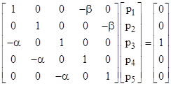
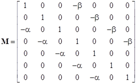
Returning to the generalized ruin problem, our example involving steps of +2 and -3 can be expressed in matrix form, and (again) without loss of generality we can re-normalize the probabilities so that the sum α(P₄ + P₅) + β(P₁ + P₂ + P₃) equals unity. The system equations in the re-normalized probabilities can then be written in matrix form as

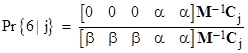
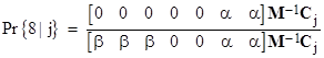
Letting M denote the coefficient matrix, and C_j the column vector whose only non-zero entry is in the jth position, the probability of “winning” from a current holding of j dollars is

This agrees with the formulas given previously, and it immediately generalizes to more complicated games with higher thresholds. For example, using the same step sizes but with a winning threshold of 8 (instead of 6), the coefficient matrix M is simply

and the probability of reaching state 8 from the jth state is

If the winning threshold is very large, and the step sizes are all fairly small, it may be most efficient to explicitly solve for the roots of the characteristic polynomial. Taking (again) our system of N = 6 and step sizes of -3 and +2 as an example, we know the probabilities are related by the linear recurrence

so the characteristic polynomial is

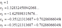
If we set α/β = 3/4 (for example), then the roots of this polynomial are

the values of the probabilities are given by

where the five constant C_j are determined by the five boundary conditions

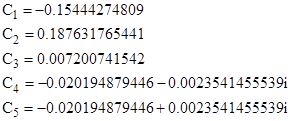
This gives the coefficients

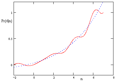
A plot of the function Pr{6|n} is shown below, along with the function consisting of just the first two terms.

For comparison, note that the value of Pr{6|3} given by this function is 0.2346870229… which is exactly the same as the value of Pr{6|3} given by equation (2) with α/β = 3/4 (which means α = 3/7) based on the closed-loop Markov model.

The above plot shows why Pr{6|2} and Pr{6|3} are so close together, as we observed previously. It also illustrates how, even for this small example, the function consisting of just the first two terms is a fairly good approximation of the actual probabilities. This approximation gets better for larger values of N, and this is true in general, so it often isn’t necessary to find all of the characteristics roots. We only need the dominant positive real root (in addition to the unit root) to give accurate results.

For a variation on this problem, see the article on Reaching Ruin in Limited Turns.

Return to MathPages Main Menu