Eigenvalue Problems and Matrix Invariants

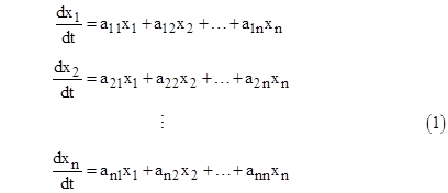
Many problems in physics and mathematics can be expressed as a set of linear, first-order differential equations in the state variables x₁, x₂, .., x_n and the time t as shown below

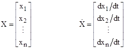
In matrix notation this system of equations can be written as

where  and X are the column vectors

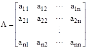
and A is the coefficient matrix

The general solution of this set of equations consists of an expression for each variable x_i as a function of time, and each of these expressions is of the form

where the coefficients c_ij are determined by the initial conditions. The values λ_i, i = 1, 2, .., n are called the eigenvalues (as the "characteristic values") of the coefficient matrix A.

The meaning of the eigenvalues can be expressed in several different ways. One way is to observe that each of the n variables in a first-order system of differential equations is individually the solution of the same nth-order differential equation, called the characteristic equation of the system. The corresponding characteristic polynomial has n roots, and these roots are the eigenvalues of the system. (The characteristic equation can be found by expressing the set of equations (1) entirely in terms of any single variable.)

Another (more common) way of looking at eigenvalues is in terms of the basis elements of the space of vector solutions to (2). For any specific one of the eigenvalues, λ_j, one solution of the system (2) is given by just taking the jth component of each variable x_i(t), giving a solution vector X(t) with components

for i = 1, 2, …, n. We can safely assume this represents a solution (though certainly not the most general solution) of (2), because the "c" coefficients of (3) are arbitrary functions of the initial conditions, and there are certainly conditions such that all but the jth coefficient of each x_i(t) is zero.

Hereafter we will denote the specific eigenvalue λ_j as simply λ. Taking the derivative of (4) gives the components of the derivative vector X′(t)

for i = 1,2,..,n. As a result, equation (2) becomes

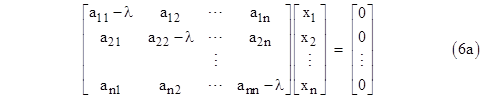
In other words, the effect of multiplying the vector X by the matrix A is to produce a rescaled version of X. (Another application of this, aside from differential equations, is in studying spatial rotations, where the vector X that is left pointing in the same direction after being multiplied by a rotation matrix A is obviously pointed along the axis of rotation.) Substituting this particular solution into the original system of equations (1) and combining terms, we have the matrix equation

Notice that the particular eigenvalue λ has been subtracted from each of the diagonal terms of the coefficient matrix. Thus, we can express the above symbolically as

where I is the nxn identity matrix

It might seem at first that the algebraic system of equations (6) can be solved simply by Gaussian elimination or any other standard technique for solving n equations in n unknowns, for any arbitrary value of the parameter λ. For example, we might try to express x_j as the ratio of the determinant of (A–λI) with the right-hand column vector substituted for the jth column, divided by the determinant of the unaltered (A–λI). However, since the right hand column consists entirely of zeros, the numerator of every x_j will be identically zero, which just corresponds to the trivial solution x_j(t) = 0 for all j. Does this mean there are no non-trivial solutions?

Fortunately, no, because there is an escape clause. Every x_j(t) is of the form 0/det(A–λI), but need not be zero IF (and only if) the determinant of (A–λI) itself is zero. In that special case, the system is singular, and each x_j(t) is indeterminate (0/0) based on the full system, and so the system degenerates, and we in general we have non-trivial solutions.

Of course, this escape clause only works if det(A–λI) = 0, which will not generally be the case for arbitrary values of λ. In general if we algebraically expand the determinant of (A–λI) we get a polynomial of degree n in the parameter λ, which is the characteristic polynomial of the system, and we need L to be one of the n roots of this polynomial. For each one of these roots (the eigenvalues of the system) we can then determine the corresponding non-trivial solution X(t). These are called the eigenvectors of the system. (It is possible for more than one vector to satisfy the system for a given eigenvalue, but we typically deal with systems in which each eigenvalue allows a unique eigenvector.)

We've now seen two ways of arriving at the characteristic polynomial of the system. The first was to algebraically eliminate all but one of the x variables from the set of equations, resulting in a single nth-order differential equation in the remaining variable, and then evaluating the characteristic polynomial of this equation. The second way is to algebraically write out the formula for the determinant of the coefficient matrix with the diagonal elements decremented by λ.

To expedite this latter approach, it's useful to note that the coefficients of the characteristic polynomial of an nxn matrix M are given by the n "invariants" of the matrix. If we write the characteristic polynomial as

then the coefficient g_j is the sum of the determinants of all the sub-matrices of M taken j rows and columns at a time (symmetrically). Thus, g₁ is the trace of M (i.e., the sum of the diagonal elements), and g₂ is the sum of the determinants of the n(n–1)/2 sub-matrices that can be formed from M by deleting all but two rows and columns (symmetrically), and so on. Continuing in this way, we can find g₃, g₄,... up to g_n, which of course is the determinant of the entire n x n matrix.

Incidentally, as was first noted by Cayley, the matrix M itself is automatically a root of its own characteristic polynomial. It's also worth noting that since (7) is also the characteristic polynomial of the single nth order differential equation satisfied by each of the variables x_j(t), the technique described in the note entitled “Root-Matched Recurrences For DiffEQs” can immediately be used to determine the coefficients q_i of the recurrence relation for any given discrete time increment Δt, giving the vector X(t) as a linear combination of the n prior vectors

Return to MathPages Main Menu