Something Like Quantum Mechanics

Suppose one of the observable attributes X of a physical system has the form of a binary variable x which can be either true or false, and suppose we have a physical law that tells us how the value of x changes with time in specified circumstances. Letting a numerical value of x = +1 signify "true" and a numerical value of x = −1 signify "false", the equation(s) expressing our physical law may be of the form x = f(t) where the function f takes on only the values −1 or +1. In this case we say the physical law ranges exactly over the observable states of the system.

However, it's conceivable that a physical law might range over a larger set than the set of observable states. For example, the function f(t) representing the physical law governing the behavior of x might range over the entire set of real numbers on the interval from −1 to +1, even though the only observable states correspond to the two specific values −1 and +1, as depicted below.

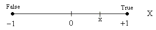
In order for the physical law to be meaningful we need some interpretation of the intermediate values of x, values which do not correspond to observable states. One possible interpretation is that the numerical value of x indicates the propensity of the system to be observed in State +1 if a measurement of the X attribute is made. If the numerical value of x is −1, 0, or +1, the probability that X will be observed in State +1 should be 0, 1/2, and 1 respectively. Naturally the probability of being observed in State −1 is the complement. This leads us to define

If we find that repeating the same measurement twice in a row invariably yields the same value each time, we may conclude that the state of the system "jumps" from the intermediate value to the observed value when a measurement is made. (Needless to say, this raises a number of questions about what constitutes a measurement.)

We define the uncertainty in the attribute X as zero if x has the value -1 or +1, and as infinite if x has the value 0. The simplest function giving these values is

It's convenient to represent these ideas by allowing the state of the system to be not just the points between +1 and −1 on the X axis, but at any of the points on the unit circle in the x,y plane as shown below.

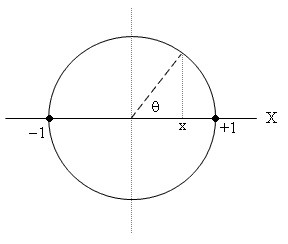
In place of the state variable x we can use the angle θ defined by x = cos(θ). Then the probability of observing the system in State +1 is [1+cos(θ)]/2 = cos(θ/2)², and the uncertainty in X is U_X(θ) = tan(θ)². In this representation each variable's real axis is accompanied by a perpendicular axis, which might be regarded as the axis of another observable variable, which we will call Y, as shown below.

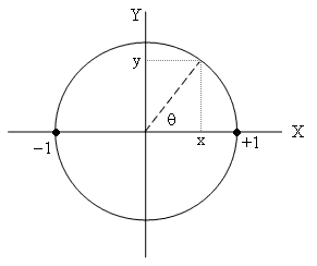
Just as with the X variable, we can also make a measurement of the Y variable, with the result being that the system jumps to +1 on the Y axis if Y is observed to be true, or −1 on the Y axis if Y is observed to be false. In terms of the parameter θ the probability of State +1 is [1+sin(θ)]/2 and the uncertainty in Y is U_Y(θ) = tan(θ + π/2)². The product of the uncertainties in the X and Y variables is therefore

This is the minimum amount of uncertainty that we can have in the joint state of these two variables, because by measuring one of them, reducing its individual uncertainty to zero, the uncertainty in the other value becomes infinite. We can imagine a measurement process that is intermediate between X and Y, essentially selecting another axis on which to project the state of the system, but after performing this intermediate measurement the product of uncertainties will still be 1.

This representation can immediately be generalized to three variables by allowing the state of the system to reside at any point on a unit sphere in three dimensions. Then depending on which measurement we perform, the system will be projected onto one of the three axes. The equations of motion (i.e., the physical laws) governing the system range over the entire surface of the sphere, but the only observable states are the six points [±1,0,0], [0, ±1,0], and [0,0, ±1]. These are the eigenvalues for rotations about the x, y, and z axes respectively.

The two non-classical features of the model described above are (1) the laws of motion range over a larger set of states than the set of observable states, and (2) some sets of observable variables are inherently inter-dependent, in the sense that they can be represented by a smaller number of state variables. Thus the system variables are over-determined in one sense and under-determined in another. They are over-determined because there are more states than observable states, but they are under-determined because there are more observable variables than state variables. For example, our original X variable has only two observable values (−1 or +1) but infinitely many state values (the real numbers from −1 to +1), and the same is true for the Y variable, but these two variables can actually be represented by a single variable, θ, so they have just one degree of freedom, not two, but this degree of freedom is continuous, not discrete.

Continuing to higher dimensions, we might represent more complex systems and variables and algorithmic laws in terms of binary variables, as with a universal Turing machine. Certain subsets of these variables could be consolidated into “spherical” relations, whereas others would be mutually independent (cylindrical spaces).

Return to MathPages Main Menu