Markov Modeling for Reliability

Part 2:  Markov Model Fundamentals

2.1  What is a Markov Model?

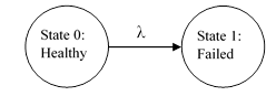
For any given system, a Markov model consists of a list of the possible states of that system, the possible transition paths between those states, and the rate parameters of those transitions. In reliability analysis the transitions usually consist of failures and repairs. When representing a Markov model graphically, each state is usually depicted as a “bubble”, with arrows denoting the transition paths between states, as depicted in the figure below for a single component that has just two states: healthy and failed.

The symbol λ denotes the rate parameter of the transition from State 0 to State 1. In addition, we denote by P_j(t) the probability of the system being in State j at time t. If the device is known to be healthy at some initial time t = 0, the initial probabilities of the two states are P₀(0) = 1 and P₁(0) = 0. Thereafter the probability of State 0 decreases at the constant rate λ, which means that if the system is in State 0 at any given time, the probability of making the transition to State 1 during the next increment of time dt is λdt. Therefore, the overall probability that the transition from State 0 to State 1 will occur during a specific incremental interval of time dt is given by multiplying (1) the probability of being in State 0 at the beginning of that interval, and (2) the probability of the transition during an interval dt given that it was in State 0 at the beginning of that increment. This represents the incremental change dP₀ in probability of State 0 at any given time, so we have the fundamental relation

Dividing both sides by dt, we have the simple differential equation

This signifies that a transition path from a given state to any other state reduces the probability of the source state at a rate equal to the transition rate parameter λ multiplied by the current probability of the state. Now, since the total probability of both states must equal 1, it follows that the probability of State 1 must increase at the same rate that the probability of State 0 is decreasing. Thus the equations for this simple model are

The solution of these equations, with the initial conditions P₀(0) = 1 and P₁(0) = 0, is

The form of this solution explains why transitions with constant rates are sometimes called “exponential transitions”, because the transition times are exponentially distributed. Also, it’s clear that the total probability of all the states is conserved. Probability simply “flows” from one state to another. It’s worth noting that the rate of occurrence of a given state equals the flow rate of probability into that state divided by the probability that the system is not already in that state. Thus in the simple example above the rate of occurrence of State 1 is given by (λP₀)/(1-P₁) = λ.

Of course, most Markov are more elaborate than the simple example discussed above. The Markov model of a real system usually includes a “full-up” state (i.e., the state with all elements operating) and a set of intermediate states representing partially failed condition, leading to the fully failed state, i.e., the state in which the system is unable to perform its design function. The model may include repair transition paths as well as failure transition paths. The analyst defines the transition paths and corresponding rate between the various states, and then writes the system equations whose solution represents the time-history of the system. In general, each transition path between two states reduces the probability of the state it is departing, and increases the probability of the state it is entering, at a rate equal to the transition parameter λ multiplied by the current probability of the source state.

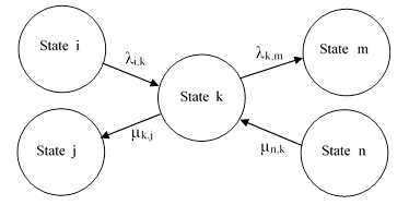
The state equation for each state equates the rate of change of the probability of that state (dP/dt) with the “probability flow into and out of” that state.  The total probability flow into a given state is the sum of all transition rates into that state, each multiplied by the probability of the state at the origin of that transition.  The probability flow out of the given state is the sum of all transitions out of the state multiplied by the probability of that given state. To illustrate, the flows entering and exiting a typical state from and to the neighboring states are depicted in Figure 1.

FIGURE 1:  Transitions into and out-of State P_k

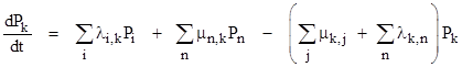
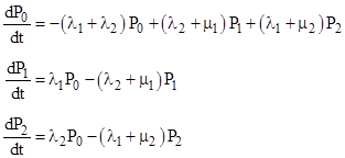
This isn’t intended to represent a complete Markov model, but only a single state with some of the surrounding states and transition paths. It’s conventional in the field of reliability to denote failure rates by the symbol λ and repair rates by the symbol μ, sometimes with subscripts to designate the source and destination states. The state equation for State k sets the time derivative of P_k(t) equal to the sum of the “probability flows” corresponding to each of the transitions into and out of that state. Thus we have

Each state in the model has an equation of this form, and these equations together determine the behavior of the overall system.

In this generic description we have treated repair transitions as if they occur at constant rates, but, as noted in the Introduction, actual repairs in real-world applications are usually not characterized by constant rates.  Nevertheless, with suitable care, repairs can usually be represented in Markov models as continuous constant-rate transitions from one state to another, by choosing each repair rate μ such that 1/μ is the mean time to repair for the affected state. This is discussed more fully in subsequent sections.

2.2  A Simple Markov Model for a Two-Unit System  

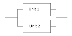
To describe the various techniques for including the effect of repairs, we will consider the simple 2-unit system shown in the figure below. This system will perform its intended function if either Unit 1 or Unit 2, or both are operational.

Simple 2-unit System

The individual units have constant failure rates of λ₁ = 50E-06 and λ₂ = 20E-06 respectively.  (All rates discussed in this article will be expressed in units of failures per hour, unless otherwise specified.) This system can be in one of four possible states, (1) both units healthy, (2) Unit 1 failed but Unit 2 healthy, (3) Unit 2 failed but Unit 1 healthy, and (4) both units failed.

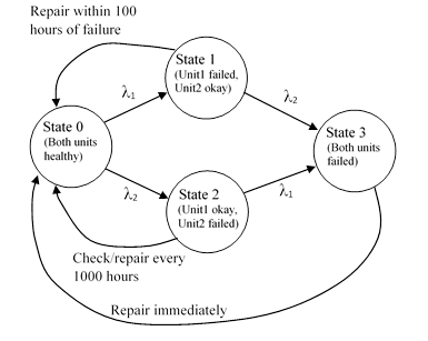
The maintenance strategy for this system is as follows: The status of unit 1 is monitored continuously and, if it fails, the operator will repair it within 100 hours of the failure. (During this period, the system continues to function, relying on Unit 2.)  The status of Unit 2 is not monitored continuously, but the operator is required to inspects it every 1000 hours, and if it is found to be failed during one of these periodic checks, it is repaired at that time. Lastly, if the overall system fails (i.e., both units are failed), both units are immediately repaired (or replaced), returning the system to the “full-up” state. This is a fairly realistic set of repair definitions for a real-world system.  When we include these repair transitions, the two-unit model can be depicted as shown below.

The immediate repair of the fully-failed state can be accurately represented by a constant-rate transition with a very large (or infinite) rate. However, the repair transitions for the two partially failed states are not strictly “Markovian”, because the repair times of Unit 1 depend on the time of failure (not just on the present state), and the repair times of Unit 2 have a discrete rather than continuous density distribution, i.e., they occur only at discrete intervals so, strictly speaking, they cannot be assigned a constant rate.

However, the repairs of Unit 1, which occur within 100 hours of failure, can be conservatively represented by a constant repair rate of 1/100 per hour. Admittedly it might be repaired more quickly, but in the absence of any data to substantiate the quicker repairs, it is usually best to just assume that the operator waits the full 100 hours before making the repair.

Likewise for the periodic inspection/repairs of Unit 2, we can always conservatively represent such repairs by a transition with a constant rate of 1/1000 per hour, because the time from failure to repair can never exceed 1000 hours. However, this may be considered excessively conservative, because it assumes every failure occurs at the very beginning of an inspection interval, so that the fault exists for nearly the full interval before being found and repaired. This would be fairly accurate if the MTBF of the unit was small in comparison with the inspection interval, but in practice this is almost never the case. To the contrary, an inspection interval for a unit is ordinarily chosen to be a small fraction of the unit’s MTBF, because we don’t want the system to be operating with latently failed units for any significant length of time. Therefore, in practice the distribution of failures in an interval is normally uniform, so the expected time between failure and repair is actually half of the inspection interval. In such cases we are justified in using a repair rate of 2/T, instead of 1/T, where T is the periodic inspection/repair interval.

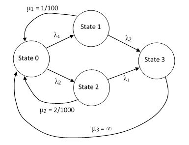
On this basis the Markov model for the simple two-unit system, including all the failure and repair transitions, is as shown in the figure below.

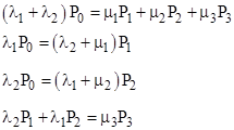
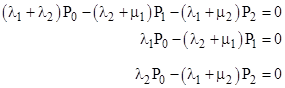
Notice that, since the repair rate of the fully-failed state (State 3) is infinite, the probability of that state will be zero, but we will leave it in the model for conceptual clarity. The total system failure rate is the total flow rate into that state, which is λ₂ P₁ + λ₁ P₂. To determine the long-term average system failure rate we need consider only the steady-state condition, i.e., the flow entering each state equals the flow exiting the state. Hence the system equations are simply

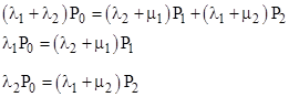
The quantity μ₃ P₃ represented by the fourth equation might seem to be indeterminate, because it equals zero multiplied by infinity. However, the left side of that equation defines the value of this quantity, which (as noted above) is the overall system failure rate. Substituting from the fourth equation into the first, we eliminate the empty state P₃, and the system equations can be written as

The second two equations immediately give

We also know that the sum of all the probabilities must always equal 1, and since P₃ = 0, the conservation equation is simply

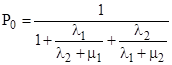
Substituting for the values of P₁ and P₂ from the preceding equations and solving for P₀, we get the steady-state value of P₀

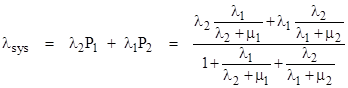
The steady-state values of P₁ and P₂ are given in terms of P₀ by the preceding equations, so this enables us to write the overall average system failure as

Inserting the values λ₁ = 50E-06, λ₂ = 20E-06, μ₁ = 1/100, and μ₂ = 2/1000, this gives the average total system failure rate of λ_sys = 5.79E-07 per hour.

2.3  Matrix Notation

The state equations for the simple system in Section 2.2 were written out explicitly and solved in an ad hoc manner, but for larger and more complicated models it is often more convenient to write the equations in matrix form and solve them in a systematic way. In general there is a state equation for each state of the model, but these equations are not all independent, because the sum of all the state probabilities must always equal 1. This constraint must be imposed in order to determine the solution. For example, the steady-state equations for the states in example in 2.2 are

but the first equation is simply the sum of the other two equations, so it is redundant. It is convenient to replace the first equation with the conservation requirement P₀ + P₁ + P₂ = 1. The resulting set of equations is solvable, and can be written in matrix form as

where

The solution is simply P = C^-1U. In general, the system shutdown rate will be some linear combination of the state probabilities. In this example, the system shutdown rate is λ₂ P₁ + λ₁ P₂, so we can define the row vector L = [ 0  λ₂  λ₁ ] and write the average system failure rate as

2.4  Delayed Repair of Total Failures

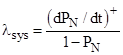
In the example of 2.2 we stipulated that a totally failed system will be repaired immediately, so the repair rate on the total failure state was infinite, and hence the probability of being in that state was zero. This was done mainly for convenience, since the actual repair rate for totally failed systems does not affect the result. We could just as well have selected some finite rate of repair for State 3, and we would have gotten exactly the same answer (provided the rate is not zero). This is because the overall system failure rate (often called the “hazard rate” in reliability literature) is defined as the rate of failure for systems that are not already failed. In other words, if state N is the total failure state, the rate of total failure is defined as

where (dP_N/dt)⁺ denotes the rate of entry into the state P_N. Thus the rate is normalized to the non-failed portion of the population, so it doesn’t matter how much time is taken to repair (or replace) totally failed units. The failure rate of operational units is not affected.

In the example of 2.2 we chose an infinite repair rate for state 3 (the fully-failed state), and therefore P₃ = 0, so the denominator of the above expression is 1, and hence the system failure rate is simply (dP₃/dt)⁺ =  λ₂ P₁ + λ₁ P₂. If we had chosen a finite repair rate for state 3, we would have gotten a non-zero value of P₃, and so we would have needed to divide λ₂ P₁ + λ₁ P₂ by 1 – P₃. However, it can be shown that the values of P₁ and P₂ would have been correspondingly affected, so that the resulting value of λ_sys was exactly the same. This is why we can set the repair rate on the total failure state to infinity, effectively reducing the number of system states by one, and simplifying the solution, without affecting the result.

2.5  Transient Analysis

In some circumstances a transient (time-dependent) analysis of the open-loop model (i.e., without repairs) is useful. For example, when determining the minimum acceptable system configuration for dispatch, and the length of time allowed for such dispatch, we may wish to know not just the average system failure rate for all possible configurations, but also the worst case instantaneous system failure rate as a function of time for a given configuration. We may also wish to know the sensitivity of the worst-case instantaneous failure rate to variations in the dispatch interval, to account for in-service waivers, and so on.

A time-dependent analysis can be conducted on either closed-loop or open-loop models, i.e., models with or without repairs. (This is in contrast with a steady-state analysis, which is meaningful only for closed-loop models, because the steady-state condition of an open-loop model is simply the fully-failed state with probability 1.)

Consider again a simple system comprised of two independent components, as discussed in Section 2.2. The full time-dependent equations (including repair transitions) are

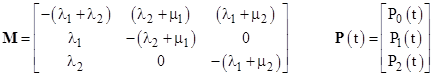
Using the matrix notation described in Section 2.3, these equations can be expressed in the form

where

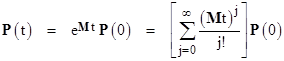
Given any initial conditions P(0), the time-dependent solution of this system of equations is simply

The instantaneous system failure rate at any time t is λ_sys(t) = LP(t) where L is (again) the row vector L = [ 0  λ₂  λ₁ ].

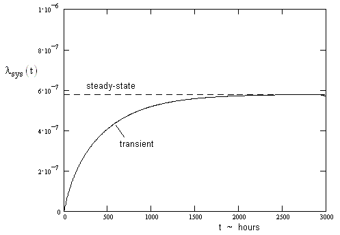
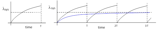
To analyze the transient behavior of the closed-loop system, we insert the failure rates λ₁, λ₂ and the repair rates μ₁, μ₂ specified in Section 2.2 into these equation. Then, beginning from a full-up configurations, the instantaneous system failure is as shown in the plot below.

The instantaneous rate has already come close to the asymptotic steady-state rate in just 1000 hours. Typically an entire fleet will operate for millions of hours, so the transient behavior during the first several hundred hours is insignificant. This is why the steady-state analysis, as described in Section 2.2, is usually adequate for determining the average system failure rate of the closed-loop system.

However, the above transient analysis assumed that the repair transition times are continuously (exponentially) distributed, whereas in fact the repairs of State 2 are periodic, i.e., the repair times have a discrete distribution. The repair rate is zero during each inspection/repair interval, and infinite for an instant at the end of each interval. (The repairs of State 1 are also not strictly Markovian, because the repair occurs a fixed amount of time after the failure, but since the entry times are continuously distributed, the exit times are as well, with an offset in time. It is generally acceptable to treat such transitions as Markovian.)

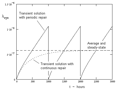
To evaluate the instantaneous effect of the periodic repairs of State 2, we need to solve the system equations with μ₂ set to zero for a period of time equal to the inspection/repair interval. Then at the end of each interval we discretely re-distribute any probability in State 2 back to the full-up state. These conditions serve as the initial conditions for the next interval. If we stipulate that all the probability in State 1 is also returned to the full-up state at the end of each interval, then every interval begins in exactly the same full-up condition, so the intervals repeat exactly, and hence it is sufficient to evaluate just a single interval. The plot below show the result of this analysis for an interval of 1000 hours.

The instantaneous failure rate with periodic repairs is a “sawtooth” function, repeating every 1000 hours. The mean value of the sawtooth is 5.75E-07 / hr, virtually indistinguishable from the steady-state value of 5.79E-07 / hr computed in Section 2.2.  Thus if our objective was only to determine the average system failure rate, there would be no benefit in doing the extra work to evaluate the time-dependent solution. On the other hand, the time-dependent solution provides the peak instantaneous failure rate, which may sometimes be of interest, depending on how the reliability criteria are defined.

2.6  Discussion

The main focus of many reliability analyses is to determine the steady-state solution of the “closed-loop” system. This is mainly because, since unlimited latency is usually not acceptable for critical systems, almost all components affecting the functionality of a critical system are monitored or inspected at fairly short intervals of time, and repaired or replaced if they are found failed. Hence the system is repeatedly restored to its fully functional state, and our main interest is in determining the long-term average reliability over many such maintenance cycles. As a result, the steady-state solution of the closed loop model (i.e., taking all repair transitions into account) is usually what the analyst needs to determine. The repeating variations within each maintenance cycle are usually not of interest.

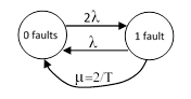
To clarify the relationship between the steady-state closed-loop solution and the transient solution (which may be either open or closed loop), consider again the simple system discussed in Section 2.2, but for simplicity assume both units have identical failure rates, denoted by λ, and suppose both units are treated in the same way for repairs. Since the two components are identical, there is no need to distinguish between the two single-fault states, so the open-loop system (i.e., without repairs) can be represented by a three-state model shown below.

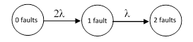
The failure of either component moves the system from state 1 to state 2, and then the failure of the remaining component move the system to state 3. (This is an example of state aggregation, discussed further in Section 3.2.) The time-dependent state equations for this open loop model are

and they give the rate of entering the “2 fault” state as

As t increases to infinity, the failure rate of this model approaches 2λ, whereas it’s well known that the renewal rate for a dual-redundant system is 2λ/3. This illustrates that the asymptotic failure rate of the open loop model does not generally represent a useful measure of system reliability. (In general, the asymptotic open-loop rate equals the largest of the eigenvalues of the system equations.)

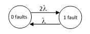
To get a more meaningful measure of system reliability, we must account for the fact that a totally failed system will be repaired or replaced. We do this by adding a transition (with infinite rate) from the “2 fault” state back to the “0 fault” state. In effect, the “2 fault” state then disappears, so the “renewal” (closed-loop) version of this problem is represented by the two-state model shown below.

The time-dependent state equations of this model are

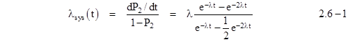
and they give the system failure rate (also known as the renewal rate) as

If we let t increase to infinity, this asymptotically approaches the long-term rate 2λ/3, as we would expect. Of course, the long-term rate could also be inferred trivially from the steady-state equation λP₁ = 2λP₀ = 2λ(1-P₁), which gives λ_sys = λP₁ = 2λ/3.

However, this model is still partially “open loop”, because we have not accounted for any repair transitions from State 1 back to State 0 (other than by passing through the total system failure state). If State 1 is actually inspected and repairs every T hours, there are two approaches we could take to incorporate these repairs into the model. One approach is to simply integrate the time-dependent equation (2.6-2) from t = 0 to T, and divide by T, to give the average rate over that interval. This gives

This approach is fairly easy for such a simple model, but for more complex models the integration of the system equations can become quite laborious.

An alternative approach is to use the steady-state method by incorporating the time limit T into the Markov model itself, as an exponential transition with constant rate. As discussed in Section 2.2, we can represent a periodic inspection/repair by a continuous transition with a rate that gives the same mean time between a component failure and repair. The appropriate value of this time is in the range from T/2 to T (depending on the magnitude of λT). Representing the periodic transition of characteristic time T with an exponential transition with constant rate μ = 2/T, the system can be represented by the model shown below.

Now that we have represented all the aspects of the problem in terms of Markovian transitions, the result is again trivially found from the steady-state condition (λ + 2/T)P₁ = 2λP₀ = 2λ(1-P₁), which immediately gives

Equation (2.6-4) gives virtually identical results as equation (2.6-3) for any λT less than 0.1 or greater than 10. Even if λT happens to be in the small window around 1, the difference between equations (2.6-3) and (2.6-4) reaches a maximum of only about 12%. For conservatism, one can always use μ = 1/T (instead of 2/T), or one can use a refined estimate of μ part-way between 1/T and 2/T. (See Section 3.1.)

In practice, both equations (2.6-3) and (2.6-4) entail idealizations that are not perfectly representative of real-world situations. Essentially they both represent many real-world situations equally well. The transient analysis represents the average instantaneous failure rate over a single period T, whereas the steady-state analysis approximates the long-term average failure rate over multiple intervals of duration T, as illustrated below.

Thus we can compute the average system failure rate over a finite time period T by either a transient or a steady-state analysis. The latter is usually much simpler and easier to perform, and provides adequate accuracy for most practical purposes. It’s also worth emphasizing that although the transient analysis is “exact”, it applies strictly to just a single interval T, as if this was the entire life of the system, whereas (as noted previously) most critical systems are maintained at regular intervals, periodically being restored to the full-up condition, so the right-hand plot in the figure above is more representative of the situation, and hence the period T usually represents a repetitive repair interval rather than a life limit. Furthermore, if T actually does represent a life limit, it is typically required to be some multiple (e.g., a factor of 3) of the actual estimated life of the system, unless the life limit is strictly enforced. In view of this, the difference between representing the interval as a discrete limit (transient analysis) or as a continuous transition (steady-state analysis) is relatively insignificant.

It’s also worth noting that the issue of discrete versus continuous repair transitions is not unique to Markov models. For example, the very same issue arises in fault trees analysis, when we assign to each basic component, with failure rate λ and exposure time T, a failure probability of (1-e^-λ^t). This represents the probability attained at the very end of the interval T, whereas the average probability during that interval is actually about half of this value, i.e., the average would be given by using an exposure time of T/2 instead of T. Nevertheless, it’s very common to use the full exposure time T in fault trees, with the understanding that this is conservative. If three events are AND’d together in a fault tree, and each of them uses an exposure time of T instead of T/2, the joint probability is conservative by a factor of 8. Similar results apply for Markov models if we simply use 1/T instead of 2/T for all the periodic repair transition rates.

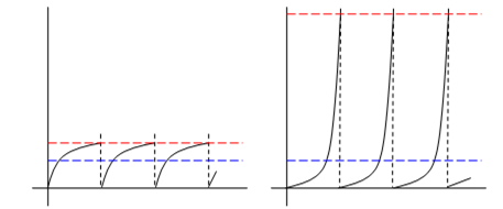
Part of the reason that this conservatism has historically been considered acceptable is that, in a sense, it is actually justified. With periodic repairs, the system’s instantaneous failure rate never converges on a single long-term value, but instead settles into a limit cycle, repeatedly passing through a band of instantaneous failure rates. The average failure rate doesn’t fully characterize the exposure, because it’s possible for two systems with identical average failure rates to have significantly different maximum instantaneous failure rates, as illustrated below.

The use of an exposure time of T (instead of T/2) for a fault tree of the left-hand system would only be conservative by roughly a factor of 2 or less, but for the right hand system it would be conservative by a much larger factor. But the analyst might justify this extra conservatism (for the right hand system) based on the fact that for this system the failure rate is a more sensitive function of the period duration. For example, if an operator forgets or defers one of the scheduled maintenance checks, the effect on the left-hand system would be minor, but the effect on the right hand system could be catastrophic. Since, in practice, inspection intervals aren’t carried out with perfect precision, it makes sense to allow for some tolerance on the value of T, and this translates into a need for more conservatism in the right-hand system. A transient analysis is one method of determining the “shape” of the instantaneous failure rate as a function of time, enabling us to assess this sensitivity. A steady-state analysis does not provide this information.

Another possible reason the analyst might want to know the maximum instantaneous failure rate is when determining the length of time that should be allowed for dispatching the system in certain degraded conditions (e.g., when operating with failures under the Minimum Equipment List), or if some limitation has been placed on the maximum allowable probability of failure for any dispatchable condition. Again, a steady-state analysis does not provide this information, so a transient analysis may be necessary in such cases. Unfortunately, for complex systems it is rarely possible to derive the exact analytical solution to the time-dependent system equations (as we did for the simple model above), so it is usually necessary to integrate the state equations numerically.

Another situation in which it may be necessary to deal with the full time-dependent equations is when dealing with a non-homogeneous Markov model. This refers to the more general class of models for which the transition rates are not constant, but instead are functions of the “ages” of the components. Models of this type are briefly discussed in Section 3.8.  Transient solutions are also of use when analyzing “phased missions”, as discussed in Section 3.9.

Part 3: Considerations for More Complex Systems