Markov Modeling for Reliability

Part 3:  Considerations for More Complex Systems

The simple method described in Section 2 works quite well for systems with just dual redundancy, and with component repair rates that are much greater than the component failure rates (which is often the case in practice).  However, for systems with triplex (or greater) redundancy, and/or for inspection/repair rates that are relatively low (i.e., long latency times), there are additional factors that must be considered when formulating and solving Markov models. Also, if we are interested in determining not just the long-term average failure rate, but the instantaneous failure rate as a function of time, we must solve the time-dependent system equations. These issues are discussed in the following sections.

3.1  Modeling Infrequent Periodic Repairs for First-Order States

In the simple example discussed in Section 2.2, a T-hour periodic inspection/repair of a particular unit was modeled as a transition with constant rate 2/T, because the failure distribution was roughly uniform during each T-hour interval, and hence the average time from failure to repair was only T/2 hours. As noted above, we could simply be conservative and use a repair rate of 1/T, but in order to minimize the conservatism in our analysis we used m = 2/T.  However, there are two important restrictions on the use of 2/T for modeling periodic repairs. 

First, the asymptotic rate of 2/T for frequent inspection/repairs strictly applies only for failure states that are a single failure away from the fully-repaired state. In practice this is often all that is needed, because many systems make use of just dual redundancy, and the failure of both redundant units represents complete system failure, so the only candidates for periodic inspection and repairs are states that are just a single fault away from the full-up state. (See Section 3.3 for higher order states.)

Second, as already mentioned, even for first order systems, if the inspection interval is large compared with the MTBF of the unit, then the average time between failure and repair approaches T, so we should use m = 1/T in such cases. For intermediate cases, i.e., cases when the inspection/repair interval is roughly the same order of magnitude as the unit MTBF, we need to determine the appropriate rate, which will be somewhere between 1/T and 2/T.  For first-order states, a T-hour periodic inspection/repair for any first-order state can be modeled as a transition with a constant rate of

where Sl denotes the sum of all the failure rates exiting the full-up state. Notice that this formula always gives a repair rate in the range from 2/T to 1/T.  This formula is valid for any inspection interval, large or small, but only for first order states.  The following section discusses how to handle periodic repairs of higher-order states.

3.2 Simplifying Higher-Order Models By State Aggregation

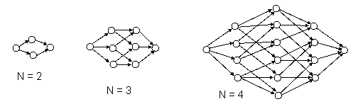
If each distinguishable condition of a system is assigned a unique state in the model, the number of states can be very large for even a moderately-sized system. To illustrate, consider a system of N identical components. If each possible combination of failures is treated as a separate state, the model will contain 2^N states, as shown in the diagrams below for N = 2, 3, and 4.

Each failure transition has the same value of l associated with it. Since all the components are identical, we can gather together all the single-failure conditions into one state, all the double-failure conditions into another state, and so on. This leads to the simpler state models with just N+1 states shown below.

In general, if two or more configurations of a system are completely symmetrical, they can be consolidated into a single state. (Section 2.6 included a simple example of state aggregation for the case N = 2.)

For another example of state aggregation, consider a system in which each channel contains operational components and protective components (e.g., tranzorbs for lightning protection) that are latent in service but that are repaired whenever the unit is serviced for some detected failure of the operational components. It might seem as if each channel should have four possible states, but in such a case only three states need to be considered, corresponding to fully healthy, protection failed, and operationally failed. This is because, for an operationally failed unit, it is irrelevant whether the protection is failed or not, because the unit will remain inoperative until it is repaired, at which time the protection will also be restored if it is failed. In effect, the operational failure and the operational-plus-protection failure states are aggregated together.

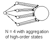
Still another example of state aggregation is when a system has a huge number of possible high-order combinations of failures, and yet only the single and double failure combinations have significant probabilities.  All the third, fourth, and higher order combinations are negligible. In such a case, it is permissible to aggregate all the higher-order states into the total system failure state, as shown in the figure below for N = 4 components.

This reduces the number of states from 16 to just 6. Since many of the higher-order combinations may actually be operational, it is conservative to lump them together with the total system failure state, but since their probabilities are believed to be negligibly small, there should be no objection to aggregating them in this way, thereby greatly reducing the number of states in the model.

3.3  Iterative Solution of Steady-State Models

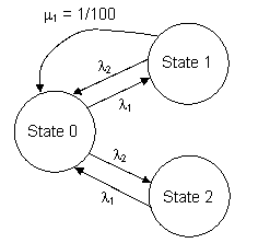
For the simple system described in Section 2.2 it was possible to recursively determine each state probability as fractions of the full-up state probability. This is because the equation for State 1 enabled us to determine the ratio P₁/P₀, and the equation for State 2 gave the ratio P₂/P₁, which could be multiplied by P₁/P₀ to give P₂/P₀. It is often the case with relatively simple Markov models that the probabilities can be computed recursively in this way. When this is possible, it eliminates the need to apply a fully general solution algorithm (such as matrix inversion) to solve the model. This is why it is often possible to easily evaluate simple Markov models by hand calculations.

However, for more complicated systems, especially those involving partial repair transitions, the state probabilities are bi-directionally interdependent, and a direct recursive solution is not possible. This isn’t an issue if a general-purpose solution algorithm is being used to invert the coefficient matrix as in 2.3, but it does present a problem for hand calculations and other “ad hoc” solution methods.

Fortunately the non-recursive effects in Markov models for reliability analysis are generally higher order (smaller) effects, so it’s possible to apply the basic recursive solution method, solving for each state probability ratio using its respective state equation as if all the other state probability ratios were known, and arrive at a first-order approximate solution. Then this process can be repeated, using the newly computed probability ratios, to arrive at an even better approximation, and so on. (This solution method has advantages over both the Gauss-Seidel method and the Jacobi method, because it exploits the homogeneous character of the system equations of a Markov model.)

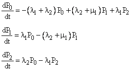
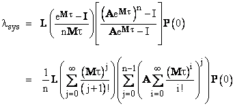
To illustrate, consider a model with the simple steady-state equations

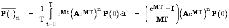
Because of the state inter-dependencies (e.g., P₁ depends on P₂ as well as P₀), this system of equations can’t be solved by direct recursion.  Note, however, that we can proceed as if the probability ratios were already known. We can divide through each equation by P₀, discard the first equation (as always, because it is redundant), and solve each of the other equations for the ratio on the diagonal. Letting Q_j denote the ratio P_j/P₀, this gives

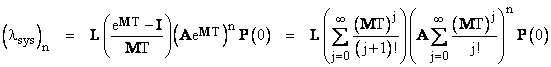
Beginning with Q₁ = Q₂ = 0, iterating these equations quickly leads to the steady-state ratios. Of course, once the ratios are known, we can compute P_j = Q_j / (1+Q₁+Q₂).  In general this approach converts the N homogeneous state equations into a non-homogeneous system of N-1 equations, which can be iterated to arrive at the solution. (They could also be solved directly, but if the purpose is to avoid the need to solve a system of equations, iteration can be used.)

3.4 Modeling Periodic Repairs for Higher-Order States

For periodic inspection/repair of states that are more than one failure away from the fully-repaired state, the equation for m given in the preceding section is not strictly applicable. Nevertheless, for some common types of higher-order models it is still possible to accurately estimate the applicable repair transition rate for representing a T-hour inspection/repair interval.

As noted previously, we always have the option of using m = 1/T, since the mean effective repair rate can’t be any lower than this. However, in many cases we can justify the use of a significantly higher rate. In fact, for higher-order states, we can often justify using a rate even greater than 2/T. This is because the rate of entry into higher-order states is not constant, but increases over time, as the probabilities of the feeding states increase. As a result, entry into a higher-order state is not uniformly distributed over the interval, it is weighted toward the end of any given inspection interval, and hence the mean time to repair may be even smaller than T/2.

For certain common types of higher-order models, the optimum rates corresponding to periodic inspection/repairs are easy to determine. For example, consider a system consisting of N identical units, each of which has a failure rate of l. The system remains operational unless all N of the units has failed. If the system fails, it is repaired immediately to the full-up state, but aside from this the only maintenance is that the system is inspected every T hours, and any units found failed are repaired at that time.  A Markov model for this system, with N = 4, is shown below.

Here we have modeled the T-hour inspection/repair as constant-rate transitions for each of the three partially-failed stated, but the rates differ because the mean times to enter the respective states are all different. In general, for a system of this type, with N identical components, it can be shown that periodic inspection/repair of a state that is k failures away from the fully-repaired state can be represented by a transition with constant rate m = (k+1)/T if the inspection interval is small compared with the unit MTBF, whereas it can be represented by a transition with constant rate m = 1/T if the inspection interval is large compared with the unit MTBF. To cover both of these regimes, and the intermediate region between them, it’s convenient to use the simple formula

However, it should be emphasized that this formula is tailored specifically for systems consisting of N identical units, with no repairs other than the T-hour periodic/inspection of all the units (along with the immediate repair of a totally failed system). In practice we may encounter more complicated systems, with dissimilar units and a variety of maintenance strategies for each unit. It is always possible to determine a set of constant values to represent the repair transition rates such that the overall system failure rate is correct, but for highly complex systems it essentially becomes necessary to carry out an exact analysis of the system in order to determine suitable repair rates for the approximate solution. Of course, once the exact analysis has been performed, there may be no need to perform an approximate analysis. Hence, for highly complex models involving periodic repair intervals of intermediate length (i.e., intervals that are on the same order of magnitude as the MTBF of the units), the approximate method of solution based on constant repair rates may not be suitable. Such models are relatively rare in practice, but when they arise, it is advisable to use one of the “exact” solution methods described in the next section.

3.5  Exact Solution of Complex Models with Infrequent Periodic Repair

The simple system discussed in Section 2.2, including the periodic repair, can be very satisfactorily modeled using the simple method described in that section. However, we will use that system to illustrate the exact solution. The first step is to consider the Markov model with all the transitions that can be accurately modeled with constant rates. We exclude the periodic inspection/repairs, on the assumption that we are not able to accurately represent those as transitions with constant rates. Thus we have the system shown below.

We have omitted the fully-failed state (State 3), because as explained in Section 2.2 that state contains no probability (because it is repaired immediately). The time-dependent state equations for this system are

It is convenient to express this set of equations in matrix notation as

where

Given any initial conditions P(t) at time t, the state probabilities at some later time t+T are given by

Now, at the initial time t = 0 we have P(0) = Transpose[1 0 0], and at the end of the first T-hour periodic inspection interval this formula gives the new state probabilities P(T). At this point we wish to inspect and repair any systems found in State 2 back to State 0. This can be accomplished by multiplying P(T) by re-distribution matrix A defined as

After the first interval T and carrying out the first inspection/repair, the state probabilities are P(T) = (Ae^MT)P(0), and after the second inspection/repair the state probabilities are P(2T) = (Ae^MT)²P(0), and so on. Therefore, after the nth inspection/repair, the state probabilities are

The average probabilities for the interval beginning at time nT is given by

where I is the identity matrix. Notice that the numerator on the right hand side is divisible by MT, so it isn’t necessary to invert the M matrix. The system failure rate is l₂P₁ + l₁P₂, so if we define the row vector L = [ 0  l₂ l₁ ], the average system failure rate during the interval beginning at t = nT can be expressed as

Inserting the values of the parameters for the example from Section 2.2, this equation shows that the system has already reached equilibrium by the end of the first 1000-hour inspection interval, at which point it is has the value l_sys = 5.84E-07.  Recall that the simple algebraic method in Section 2.2 gave the value l_sys = 5.79E-07. This confirms that, for this simple system, the algebraic method is quite adequate.

Note: Some analysts prefer to numerically integrate equation 3.5-1 rather than making use of the explicit closed-form solution 3.5-2. The results are the same.

3.6  Exact Solution With Multiple Distinct Periodic Repair Intervals

The example discussed in the preceding section involved only one periodic inspection/repair interval. The solution can be generalized to any number of distinct repair intervals. For example, suppose we have a system for which some of the components and inspected and (if failed) repaired every t hours, whereas the remainder of the components are inspected/repaired only once every T = nt hours. In other words, the longer interval is n times the smaller interval. For this system we have two “re-distribution matrices”, which we may call A and B. The first represents the repair of the t-hour components, and the second represents the repair of all components (because everything is checked and repaired at the longer interval T). It can be shown that the average system failure rate is

We note that the B re-distribution matrix doesn’t appear in this expression, because B represents complete restoration of the system to the full-up state, so, beginning from the full-up state, we need only evaluate the system reliability over n of the t periods using the A matrix. At this point the B re-distribution would restore everything to the full-up state, so all subsequent iterations would be identical to the first.

To illustrate, consider again the sample system of Section 2.2, but suppose Unit 1 did not contain continuous health monitoring (so m₁ = 0), and instead it was maintained by a periodic inspection/repair every t = 200 hours. As before, Unit 2 is inspected and repaired periodically every T = 1000 hours. Thus we have n = 5, and the coefficient and re-distribution matrices are

Since the B matrix represents complete restoration of the system, we can use the preceding equation to evaluate the average system failure rate of one complete T-hour interval (which consists of five t-hour intervals). Inserting these matrices into the preceding equation gives l_sys = 5.85E-07, which is nearly identical to the previously-computed results. This was to be expected, because the inspection of 200 hours for Unit 1 is essentially equivalent to the previous system that required repair of Unit 1 at 100 hours after failure. Recalling that a frequent periodic inspection and repair every T hours gives a mean repair time of T/2, these two maintenance strategies give the same result.

3.7  Model Truncation and Completeness

One of the main difficulties for any kind of comprehensive reliability analysis is that the number of distinct system states may grow quite large as the number of components increases.  A system consisting of N basic components has 2^N possible states (even without taking the order of occurrence into account), so any analysis method must somehow accommodate this exponential growth in complexity as the number of basic components increases. This applies regardless of the method of analysis (e.g., fault tree, Markov model, etc.). However, in practice this problem is often mitigated by the fact that the systems to be analyzed are not fully general, partly because they have been specifically designed to isolate redundant functional paths and avoid “common mode faults”. This not only is sensible design practice, it also tends to make systems easier to analyze, because groups of related components can be lumped together into a much smaller number of independent high-level partitions.

In addition, the failure probabilities of practical components tend to be many orders of magnitude smaller than 1, so combinations of more than two or three failures are often found to be negligible. It is often possible to greatly simplify an analysis by exploiting these special aspects of practical systems. However, care must be taken not to assume, in advance, that a particular system can be simplified in these ways. Meaningful substantiation of the extremely high levels of reliability (e.g., one per billion hours) mandated for safety-related systems requires a commensurate level of reliability in the analysis method, so it is not permissible to employ a method that gives the right answer for “almost all” systems. Every possible combination must be taken into account (though not necessarily explicitly), either in the design phase or in the analysis phase. This highlights the importance of applying good design practices, including strict isolation of redundant functional paths, so that systems are amenable to rigorous analysis. 

Of course, the requirement to account for all combinations doesn’t means that each combination must be explicitly represented in a model. For example, if all combinations of three or more failures are believed to be negligible, it is reasonable to include only the single and double failure combinations explicitly in the model, provided all further failure transitions from the double-failure states are routed to the complete system failure state. This will be conservative, but the conservatism will be negligible – assuming all the higher-order combinations are indeed negligibly small. If the model turns out to be overly conservative, then it will be necessary to model the higher-order combinations to justify a less conservative analysis.

It’s also worth noting that modern computers have greatly increased the size of the models that can be easily analyzed. Nevertheless, the potential for exponential growth in the number of states ensures that there will always be incentive to limit the number of states that are explicitly represented in a model.

3.8  Models with Variable Transition Rates

In most common Markov models the transition rates are constants, so the transition times are exponentially distributed (as discussed in the Introduction). It is, however, possible to construct models with non-constant failure rates. The governing state equations are the same, except that each rate l is allowed to be a function l(t) of the time. The need for variable failure rates arises in practice to account for things like “wear-our” or “infant mortality”. Of course, in order for the failure rate to correlate with such variations, the time parameter t must represent the age of the component. This is quite different from common Markov models, in which the time variable t is arbitrary, i.e., we can set t = 0 at any instant, and the system equations are valid. This is why common Markov models are said to be “homogeneous in time”, whereas if the state equations are valid only if t represents the age of the unit, the model is said to be “non-homogeneous in time”.

One of the main difficulties in dealing with variable failure rates is that a “state” is no longer fully determined by the health status of a finite number of components. The state also depends on how much time has passed since the last time each of the components was replaced or restored to it’s “as new” condition. Even if we agree to begin the model with all new components in the full-up state, a system with repairs will involve units that have failed and then been returned to the full-up state at various times, so very quickly each state will consist of a mixture of systems, all in the same operational condition, but with components of different ages (and therefore different instantaneous failure rates). Consequently, the life of each individual component must essentially be analyzed separately, with no interactions or repairs.

For example, it would not be possible to use variable failure rates in the simple two-state closed-loop model discussed in Section 2.5, because of the mixed ages of repaired and never-failed units in the full-up state. With ordinary Markov modeling techniques the most we could do is evaluate the open-loop model discussed at the beginning of that section. However, after much labor, we would find that the state probabilities are just the products of the individual component probabilities, since the two units are simply following their own individual failure rates. The application of conventional “Markov modeling” to such system’s is of little benefit.

There do exist, however, techniques for applying non-trivial Markov modeling to system with variable failure rates. One “brute force” approach is to use a Monte Carlo simulation, generating a large number of (simulated) systems and tracking them through their life cycles. Each unit is failed at a rate depending on the age of that particular unit (since it’s last overhaul). A more analytical approach is to actually model the time dependence of the failure rates by means of a sequence of states. A description of these methods is outside the scope of this document.

3.9  Phased Mission Analysis

Some missions are split into distinct phases with different configurations and/or failure modes or effects. For such missions a Markov model can be developed for each phase, and the final conditions for one phase may be used as the initial conditions for the next. Phased missions are somewhat uncommon in industry. No fundamentally new ideas are required to analyze such missions.

Part 4: Examples