Reconstructing Brouwer

Any continuous mapping of a compact convex set into itself contains at least one fixed point. In other words, given any continuous function f(x) of an n-cell into itself, there exists at least one point x₀ such that f(x₀) = x₀. This is known as Brouwer's fixed-point theorem, and it has been used to establish fundamental existence theorems in many different branches of mathematics (e.g., the theory of differential equations).

L. E. J. Brouwer (Luitzen Egbertus Jan, 1881-1966) was a Dutch mathematician and the founder of intuitionism, a philosophy which admits only things that can be constructed by finitary means. In particular, intuitionism does not accept the validity of the Law of the Excluded Middle, nor the Axiom of Choice. Ironically, Brouwer is best known (outside the philosophy of mathematics) for his fixed-point theorem, which he proved by means of conventional (non-constructive) analysis, i.e., techniques that he philosophically considered to be questionable if not downright invalid.

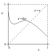
For a simple one-dimensional interval, the fixed-point theorem is fairly obvious, because any continuous function x' = f(x) of an interval, say from 0 to 1, into that same range must somewhere meet the line representing x' = x, as illustrated below.

Notice that we can assert the function x' = f(x) crosses the line x' = x for an arbitrary continuous function f, even without explicitly constructing the point of intersection. In fact, if f(x) is a higher algebraic or transcendental function, it may be impossible to give a strict finite construction of the fixed point, but we can nevertheless assert its existence -according to conventional mathematical principles.

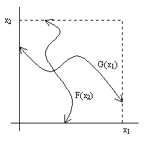
A two-dimensional n-cell can be represented as the Cartesian product of two unit intervals of this same type, which we can denote by x₁ and x₂, and the function can be split into two components x₁' = f₁(x₁,x₂) and x₂' = f₂(x₁,x₂). From the one-dimensional case we know that for any given value of x₂ there exists at least one value of x₁ such that x₁ = f₁(x₁,x₂). If there was always just one such value of x₁ for any given x₂ , the existence of an overall fixed point would follow immediately. To show how, let F(x₂) denote this (putatively unique) fixed value of x₁ for any given x₂. Clearly F must be a continuous function of x₂, so the composite function x₂' = f₂(F(x₂),x₂) is a continuous function of x₂, and hence we can invoke the one-dimensional case again to assert the existence of a value of x₂ such that x₂ = f₂(F(x₂),x₂), which is a completely fixed point. Of course, we could also have proceeded in the opposite direction, defining a function G(x₁) that gives the (putatively unique) fixed value of x₂ as a function of x₁. On a simple two-dimensional plot, the function x₂ = G(x₁) must pass continuously from the left edge to the right end of the cell, and the function x₁ = F(x₂) must pass continuously from the top edge to the bottom edge, and the argument is that they must intersect at some point, as illustrated below.

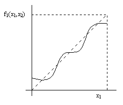
However, this argument is not adequate, because for any given value of x₂ there may be more than one value of x₁ such that x₁ = f₁(x₁,x₂), and the number of such fixed values may change as we vary x₂, so we cannot automatically claim single continuous functions F and G passing between their respective edge pairs. Therefore, in order to prove that there is a point of intersection we must consider the multi-valued functions more carefully. In general, for any given value of x₂, the function x₁' = f₁(x₁,x₂) can have multiple fixed points, as illustrated below.

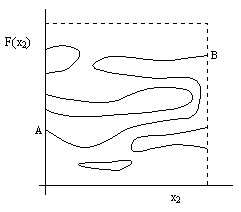
Furthermore, as x₂ is varied, this curve can shift and change shape in such a way that some of the fixed points "disappear" and others "appear" elsewhere. The four discrete corner-points can easily be treated separately, so we need consider only single-valued functions f₁ and f₂ that map to the interiors of the intervals. For such functions the number of times the function f crosses the diagonal is obviously odd, and the fixed points "appear" and "disappear" in pairs when two of them coincide. Of course, each simple crossing represents one distinct fixed point, whereas any occurrence (including contiguous spans) of the function being tangent to the diagonal is counted as either zero or one crossing accordingly as the function departs from the diagonal on the same side or on opposite sides. These observations suffice to establish the topology of the locus of fixed points. A plot of the multi-valued function F(x₂) of the x₁ fixed points as a function of x₂ for an illustrative case is shown below.

Notice that we cannot simply select the lowest fixed point, or the highest fixed point, or any other locally identifiable one of the fixed points at any given x₂, because those can change discontinuously, and therefore don't yield a continuous curve. However, notice also that at each value of x₂ there is an odd number of x₁-fixed points, and this implies that there is a continuous path extending all the way from the left edge to the right edge. (In the figure above, we have the path from "A" to "B".) This is because any closed loop, and any path that starts and ends on the same edge, has even parity, i.e., contributes an even number of crossings at each x₂. Only paths that start at one edge and end at the other have odd parity, so it follows that there must be an odd number of curves that extend continuously (though not necessarily single-valued) from one edge to the other. As a result, we are assured of an intersection between this (multi-valued) function F and the corresponding function G (since G similarly includes a contiguous path from the top edge to the bottom edge). In effect, the argument is the same as before, when we assumed single-valued F(x₂) and G(x₁) functions, except that now we parameterize these as multi-valued functions along the continuous curve (such as from A to B) that extends from one edge to the other.

Higher dimensional cases follow by direct extension of this argument. For example, in three dimensions we have three continuous functions x₁' = f₁(x₁,x₂,x₃), x₂' = f₂(x₁,x₂,x₃), and x₃' = f₃(x₁,x₂,x₃), and for any given x₂ and x₃ we can define F(x₂,x₃) as the parameterized x1-fixed point curve, i.e., a continuous curve of x₁ values such that x₁ = f₁(x₁,x₂,x₃). This allows us to "eliminate" x₁ and reduce the problem to the two-dimensional case given by x₂' = f₂(F(x₂,x₃),x₂,x₃), and x₃' = f₃(F(x₂,x₃),x₂,x₃). (Visually we can imagine the continuous multi-valued sheet of x₁ fixed points as a function of x₂ and x₃, and the sheet of x₂ fixed points as a function of x₁ and x₃, and the sheet of x₃ fixed points as a function of x₁ and x₂. Since there is at least one complete sheet in each direction that bifurcates the n-cell along that axis, these three sheets unavoidably have at least one point of intersection.) Continuing on in this way, the general result for all n follows.

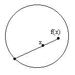
The usual proof of Brouwer's fixed-point theorem makes use of some machinery from simplical homology theory. First we establish that there does not exist a "retraction" of an n-cell onto its boundary, which is to say, there is no continuous mapping from an n-cell to its boundary such that every point on the boundary maps to itself. Given this, Brouwer's fixed-point theorem follows easily, because if x and f(x) are everywhere distinct in the n-cell, we can map each point x unambiguously to a point on the boundary by simply projecting along the ray from f(x) through x to the boundary, as illustrated below for a disk.

This mapping is continuous, and every point on the boundary maps to itself, so the mapping is a "retraction", which contradicts the fact that no retraction of an n-cell exists. Of course, we haven't actually shown this yet. The proof of the no-retraction theorem is not trivial. To prove it, first recall that a homotopy between two mappings f(x) and g(x) can be represented by a function H(x,t) that is continuous in both x and t, and such that H(x,0) = f(x) and H(x,1) = g(x). In other words, the parameter "t" serves to smoothly interpolate from f(x) to g(x). Now suppose there exists a retraction R(x) from the interior of a unit sphere (for example) to its boundary, and consider the parametric family of mappings given by H(p,t) = R((1–t)p) where "p" is a unit vector corresponding to an arbitrary point on the boundary of the unit sphere. Thus H is a family of mappings from the surface of a unit sphere into itself, parameterized by t. With t = 1, we have H(p,1) = R(0), meaning that every point on the surface maps to a single point. On the other hand, with t = 0 we have H(p,0) = R(p), meaning that every point on the surface maps to itself. These facts enable us to rule out the existence of the retraction R(x), because a singular mapping f(p) = p₀ cannot be homotopic (i.e., cannot be related by a homotopy H) to the identity mapping g(p) = p. In other words, we cannot smoothly interpolate between a singular mapping and the identity mapping.

The last assertion may be fairly intuitive, but to establish it rigorously requires some effort. In general, Brouwer characterized mappings from one n-sphere to another according to the number of times the image of former wraps around the latter. He called this integer the degree of the mapping. For example, the identity mapping f(p) = p of points on the surface of a sphere has degree 1. On the other hand, we could define a mapping such that two points on the source sphere map to each single point on the destination sphere, and the degree of such a mapping would be 2. The degree of a singular mapping f(p) = p₀ is zero, because the image of the source sphere does not wrap around the destination sphere at all. Brouwer then proved that if two mappings from one n-sphere to another are homotopic, they must be of the same degree, which is the result needed to complete the classical topological proof of Brouwer's fixed-point theorem. Incidentally, H. Hopf subsequently proved the converse, i.e., if two mappings from one n-sphere to another have the same degree, they are homotopic.

Notice that Brouwer's topologic proof of the fixed-point theorem is non-constructive, just as was our earlier algebraic proof. It posits a mapping with no fixed point, and then deduces a contradiction, proving that no such mapping is possible, but it does not give a constructive procedure for actually determining a fixed point for any given mapping... or does it? Ron Maimon proposed the following constructive analog of Brouwer's fixed-point theorem:

Given any uniformly continuous map from the disk to the disk, and any ε > 0, there exists a point which is not moved by more than ε from it's original position.

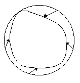
As a proof of this assertion for any continuous map f(x), he asks us to consider the value of the vector field x-f(x) along the boundary of the disk. He asserts that the vector must point inward at every point. (We should perhaps note that it's possible for a point on the boundary to map to a point on the boundary, so the vector need not be strictly inward.) Therefore the image of boundary is another closed curve in the interior of the disk, as illustrated below.

As we proceed around the boundary of the disk we can keep track of how the direction of the vector field changes, like the hand of a clock, and count how many times this hand rotates as we complete one trip around the boundary. Call this integer the winding number. To make this procedure finitistic and constructive, Maimon proposes to split up the boundary into segments of size δ, small enough so that the vector field is constant to a precision of ε over each segment. (This actually requires a limitation on the scale of variations, since otherwise we could never be sure of having identified a sufficiently small scale for the evaluations.) The winding number ought to be –1 (i.e., the vectors rotate once around in the clockwise direction.) He argues that the only way we can fail to determine the winding number unambiguously is if there is a point where the magnitude of the vector field is so close to zero (i.e., within ε of zero) that we cannot establish its direction, but in that case we have found a point that is moved less than ε under the mapping, so we are done. Assuming we have found an unambiguous non-zero winding number around the loop, we then cut the enclosed region in half, and evaluate the winding numbers around the loops enclosing these two halves. If we assume the mapping is single-valued (which precludes non-simple loops in the image), the winding number around each region must be either 0 or -1, and since the sum of the winding numbers for the partitions equals the winding number around the total region, we must have one half with a winding number of 0 and the other with a winding number of -1. Taking the latter, we can split it in half, and repeat the process. Eventually we must either reach a stage where we are unable to evaluate the winding number because of the presence of an ε-fixed-point, or else we must converge on a region smaller than ε with winding number -1, which Maimon argues must contain an ε-fixed-point.

This procedure is clarified by considering the 1-dimensional case of the Brouwer theorem, i.e., the intermediate value theorem. We bisect the interval and check to see which half still satisfies the original conditions of the problem. Eventually we reach a stage where we cannot decide up to our limit of resolution, and we declare that the midpoint of that interval is a fixed point. So we are done. But does this constitute a valid constructive argument?

According to the constructivist point of view, arguments of the "either/or" are not automatically accepted, because one of the basic tenets of constructivism is the rejection of the free use of the "law of the excluded middle". A well-known example is the "proof" that there exist irrational numbers x and y such that x^y is rational. We start with the algebraic identity

We know that the square root of 2 is irrational. Also, either the quantity in square brackets is rational or it is not rational. If it's not rational, then the above identity proves the result. On the other hand, if it is rational, then the fact that it is rational proves the result. Thus, one way or the other, there exist two irrational numbers x,y such that x^y is rational. However, we have not provided a finite procedure for determining which of the options actually leads to the x,y in question, so we haven't really constructed an example. We have only "proved" that such an example must exist, so this is not regarded as a valid constructive proof.

What does this imply for Maimon's version of Brower's fixed-point proof? His algorithm proves that any of the possible outcomes of the "algorithm" must lead to an ε-fixed point, but it doesn't tell us which of these outcomes must occur. On the other hand, Maimon's algorithm is explicitly finite, so it can be said to conform to the constructivist requirements. This is possible because Maimon is not actually proving Brouwer's fixed point theorem, he is proving the ε-fixed-point theorem. He argues that this is the only meaningful form of the theorem, because "there is no constructive definition of irrational numbers anyway, except for a small number of special cases". This is important, because the actual fixed point (in the classical sense) may have irrational coordinates, which could obviously never be determined in a finite number of steps.

Clearly, the most this algorithm can do (in a finite number of steps) is to narrow the range of possibilities down to what remains an infinite set. It seems that constructivism must assume the universe of concepts has an absolute scale, relative to which the concept of "sufficiently small" can be defined. Lacking that, all finite regions are in a sense equivalent, so knowing a fixed point is within a certain region is no more constructive than knowing that either

is a pair of irrational numbers [x,y] such that x^y is rational. On the xy plane this "construction" has narrowed down the location of [x,y] to a set of measure 0 (actually just two points). Why isn't this as good as saying we have "constructed" a fixed point to accuracy epsilon? It can only be the absolute distance between these two points that causes us to be dis-satisfied with the reduction.

Also, it's important to recognize that Maimon's guarantee of an ε-fixed point in a finite number of steps was proven classically, not intuitionistically, since it relies on the truth of statements of the form A or B without proving either A or B. In addition, the procedure gives us no assurance that we have defined a sufficiently small scale δ to resolve the variations in the mapping. In other words, we are presumably required to adopt some finitistic definition of continuity, with an absolute scale. This is indeed what Maimon was proposing, based on ideas about quantum effects in physics, but whether this is a valid foundation for a mathematical argument is debatable.

Perhaps most importantly, we should ask if it is legitimate to simply dismiss any consideration of the true fixed point by declaring that infinite precision is meaningless. Suppose we perform the algorithm to an accuracy of ε, and we verify a fixed point at that accuracy. What does that tell us about the result of the algorithm if carried out with accuracy of ε/10⁶? Are the two results necessarily close, or might we get a completely different point if our ε was different? It's not difficult to give examples, even in one dimension, of functions with very low slopes, such that many point are almost fixed points (i.e., they are ε-fixed points) without actually being fixed points. I've heard that Brouwer himself, when he became a constructivist, stopped believing his theorem; is this why?

Incidentally, there exist well-known "constructive" proofs of Brouwer's theorem, based on Sperner's coloring lemma. In one dimension, this lemma says that if we have a line segment subdivided into smaller segments, and if we color the left-most vertex red, the right-most vertex green, and use red or green for each interior vertex, then there is an odd number of segments with one red and one green vertex.

In two dimensions, we begin with a large triangle, and we sub-divide it into smaller triangles such that no vertex is in the middle of an edge of some other triangle except for the edges of the original large triangle. Now color the three outer corner vertices red, blue, and green respectively. Then color the vertices along the edges of the original large triangle, using on each edge only the colors of the two end vertices of that edge. Then color the interior vertices arbitrarily using the three colors. Sperner's lemma tells us that there is an odd number of triangles with red-blue-green vertices. To prove this, construct the "dual" graph, with a dot inside each sub-triangle, one outside each outer edge, and connect two adjacent dots if the edge between them has two distinct colors. Degree counting will show there is an odd number of degree-3 vertices on the inside. This can be extended by induction to higher dimensional cases.

To see how this can be used to prove Brouwer's fixed point theorem, consider the triangle T given in R³ by {(x,y,z)|x+y+z = 1 and x,y,z ≥ 0}. Triangulate T to ε-sized triangles. (In higher dimensions this can always be done by barycentric subdivision.) Color a vertex (x,y,z) red if (u,v,w) = f(x,y,w) satisfies u ≤ x, else blue if v ≤ y, else green if w < z. (In case of definition failure here, we have a fixed point.) By Sperner's lemma we know that there is a sub-triangle with red-green-blue vertices, so we can iterate this procedure, letting ε approach 0, to give smaller and smaller red-green-blue triangles. By compactness, there's a convergent subsequence of their first coordinates, and the limit is a fixed point.

Of course, this limiting process is not constructive (approximate reals are all we can get in the usual computational models). However, Arnaldo Mandel comments that, within the confines of constructive definitions, we can modify this proof to make it acceptable to a constructivist. Choose a point separated from the green vertex by the red-blue edge. Color that point red, and join it by a line segment to each of the colored points in that edge. Now form the "dual" graph (we don't need the dots outside the outer edges). The edge joining the new point to the blue corner belongs to a triangle, whose dot has degree one in this graph. It's not hard to see that it lies in a component which is a simple path, and the other end of the path is the triangle we seek, so we need only follow the path. This idea of proof generalizes quite directly to any dimension ≥ 2, with no need for induction.

Return to MathPages Main Menu