Combining Probabilities

Suppose Mr. Smith, who is correct 75% of the time, claims that a certain event X will not occur. It would seem on this basis that the probability of X occurring is 0.25. On the other hand, Mr. Jones, who is correct 60% of the time, claims that X will occur. Given both of these predictions, with their respective reliabilities, what is the probability that X will occur?

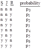
Essentially the overall context has 3 parameters, S (Smith's prediction), J (Jones's prediction), R (the real outcome). Thus, letting "y" and "n" respectively denote X and not X, the eight possibilities along with their probabilities are

where

Also, since S = R at 75% of the time, we have

and since J = R at 60% of the time, we have

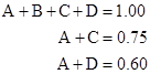
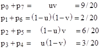
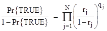
From this we want to determine the probability that R = y given that S = n and J = y. Thus, we need to find the value of p₃/(p₂ + p₃), which is the probability of [n y y] divided by the probability of [n y *], where "*" indicates "either y or n". Clearly the problem is under-specified. Setting A = p₀ + p₇, B = p₁ + p₆, C = p₂ + p₅, and D = p₃ + p₄, the conditions can be written as

which is three linear equations in four unknowns (with the extra constraint that each probability is in the interval 0 to 1), so there are infinitely many solutions. For example, we can set A = 0.5, B = 0.25, C = 0.15, and D = 0.10, and satisfy all three equations, but we could also set A = 0.6, B = 0.25, C = 0.15, and D = 0.00. Furthermore, even if we arbitrarily select one of these solutions, there are still infinitely many ways of partitioning C and D to give the values of p₂ and p₃.

For example, suppose we take the solution with C = 0.15 and D = 0.10. We then have  p₂ + p₅ = 0.15  and  p₃ + p₄ = 0.10. If we take p₄ = 0.10 and p₅ = 0.00, we have p₃ = 0.00 and p₂ = 0.15, so the probability of X is 0. On the other hand, we can equally well take p₄ = 0.00 and p₅ = 0.15, which gives p₃ = 0.10 and p₂ = 0.00, so the probability of X is 1. Thus, any answer from 0 to 1 is strictly consistent with the stated conditions.

Nevertheless, in real life the problems we confront are often (always?) underspecified, but we must still make decisions. Are there any "reasonable" assumptions we could make, in the absence of more information, that would enable us to give a "reasonable" answer? One approach would be to estimate (guess) how much correlation exists between the correctness of J and S. For example, since S seems to be smarter than J, we might assume that S is correct whenever J is correct, as well as being correct on some experiments when J is incorrect. This would imply that p₃ = p₄ = 0 and p₂ > 0, so the probability of X is 0.

Another approach would be to assume that the correctness of S and J's predictions are statistically independent, in the sense that they are each just as likely to be right regardless of whether the other is right or wrong. This assumption implies

and

Letting u = 0.6 and v = 0.75 denote the probabilities of correctness for Jones and Smith respectively, these equations together with the previous constraints uniquely determine the four sums

but this still doesn't uniquely determine the value of p₃/(p₂ + p₃). We need at least one more assumption. I would suggest that we assume symmetry between "y" and "n". In other words, assume that probability of any combination is equal to the probability of the complementary combination, given by changing each "y" to an "n" and vice versa. This amounts to the assumption that X (the real answer) has an a priori probability of 1/2, and that the probability of predicting correctly is the same regardless of whether R is "y" or "n". On this basis we have p₀ = p₇, p₁ = p₆, p₂ = p₅, and p₃ = p₄, so we have p₂ = 6/40, p₃ = 3/40, and p₃/(p₂ + p₃) = 1/3.

Therefore, assuming S and J are not correlated, and assuming "y" and "n" are symmetrical, the probability of X, given that S[75%] says X will not occur and J[60%] says it will, is 33.3%. Any (positive) correlation between S and J would tend to lower this probability.

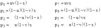
Notice that our resulting value for the probability of X is not equal to the a priori value of 1/2 that we assumed by imposing symmetry between "y" and "n". If we have some a priori reason to believe the probability of X is something different than 1/2, we could re-do the calculation using this value. (Of course, we cannot use the computed probability of X for the particular conditions at hand, because the a priori probability of X applies to all possible conditions, not just when Smith says it won't occur and Jones says it will.) To account for this additional information (if we have it), we can let x denote the a priori probability of X, and then write the individual state probabilities as

On this basis the probability of X is

Naturally if we have no knowledge of the a priori probability of X, we just assume x = 1/2, and this formula reduces to the one given previously.

For a slightly more complicated case, suppose Mr. Red's ability to correctly identify the outcome of a TRUE/FALSE experiment is 75%, Mr. Green's is 60% and Mr. Blue's is 55%. If Mr. Blue, Mr. Green, and Mr. Red all agree that the outcome of the experiment is TRUE, is the resulting probability of "TRUE" 75% or is it weighted somewhere between 75% and 55% ?

Again this is underspecified, but if we impose the assumptions of (1) pairwise independence and (2) "y"/"n" symmetry, then in the general case of N prognosticators these two assumptions are sufficient to uniquely determine the answer. In other words, if N people with reliabilities r₁, r₂, ..., r_N have each predicted the outcome will be 'TRUE', and if we assume the correctness of their predictions have no correlation, and that there is symmetry between TRUE and FALSE outcomes, then the probability of a "TRUE" outcome is

Thus, in the particular example described above with r₁ = 3/4, r₂ = 3/5, and r₃ = 11/20, the probability of "TRUE" is 11/13 (i.e., about 84.6%).

Let Q = [q₁, q₂, ..., q_N] denote a logical vector (i.e., each component q_j is either +1 for "TRUE" or −1 for "FALSE") and let Q' denote the negation (logical complement) of Q. Also, define

and let F(Q) denote the product of f(r_i, q_i), i = 1 to N. Then the probability that the outcome will be TRUE given the predictions Q is given by

Incidentally, a more perspicacious (but equivalent) way of expressing these relations is

These results are formally correct, given the stated assumptions, but as discussed earlier, the most important thing to realize about these problems is that they are underspecified and have no definite answer. For example, if the a priori probability of the outcome "TRUE" is known to be x, then the above formula becomes

Given various sets of assumptions, all of which satisfy the stated conditions of the problem, the correct probability can have any value from 0.0 to 1.0.

The formula P = F(Q)/[F(Q) + F(Q')] is valid only for one specific set of assumptions, and those assumptions are not particularly realistic. It assumes that the correctness of Smith's predictions is totally uncorrelated with the correctness of Jones's predictions, which would almost certainly not be the case in any realistic situation. (It's much more likely that Jones and Smith use at least some of the same criteria for making their predictions). To really answer the original question we would need to supply more information, specifically, the probabilities of each of the eight possible combinations of predictions and outcomes, as discussed previously.

For another example, suppose the Yankees and the Red Sox are playing, and the Red Sox have won 70% of their games, and the Yankees have won 50% of their games. What is the probability that the Yankees will win? Again the context is clearly underspecified, because the conditions of the question can be met by many different contexts, leading to many different outcome distributions. However, if we need to assign a probability based on this information alone, it's clear that our answer must assume the probability of Y beating R is some function of y and w (the fraction of games won by Y and R respectively).  Thus we need a function F(y,r) such that

It follows that

and 0 ≤ F(x,y) ≤ 1 for any x,y in [0,1]. One class of functions that satisfies this requirement is

where f is any mapping from [0,1] to [0,+inf]. For example, suppose y = 0.5 and r = 0.7.  Taking f(x) = x this gives Y a 41.7% chance of winning and R a 58.3% chance of winning. More generally, if we set f(x) = x^k and reduce the exponent k so it approaches 0, the probabilities approach 50/50, whereas with k greater than 1 the probability of Y winning goes to zero.

What is the "best" or optimal choice for f(x)? We might assume each team has a "skill level", and this level is distributed binomially. Then, given the percentage of games won by a certain team we could infer the skill level by integration over the whole population, assuming that each team plays every other team the same number of times, and assuming Pr{i beats j} = s_i/(s_i + s_j).

Another approach is to use the expression (Y)(R)/[(Y)(R) + (Y')(R')], where Y' and R' are the conjugates of Y and R. The two possible outcomes are Ywins-Rloses, and Yloses-Rwins. To find the probability (only from w/l record) of R winning we would then have

This formula has a certain aesthetic appeal, but it also has some possibly counter-intuitive consequences.  For example, suppose the two best teams in the league, X and Y, win x = 99% and y = 97% of their games, respectively. We might expect these two teams to be fairly evenly matched, which would be consistent with the formula

In contrast, the alternative formula gives

It isn't obvious that a 99% team should be this heavily favored over a 97% team. If this really was the applicable formula, then the presence of a 99% team in the league would almost preclude the existence of a 97% team, depending on how many teams are in the league and how often these teams play each other.

One possible objection to the simple weighting function f(y)/[f(y) + f(r)] with f(x) = x is that it seems the "system" will tend towards equilibrium. For systems of more than two teams, the teams will always come to equilibrium regardless of the initial conditions. In other words, each team would converge to the same win/loss record. On the other hand, a team with a winning percentage of 0.800 will have ample opportunity to sustain their winning ways by using the alternative expression

as a model. It's a good idea to impose the overall equilibrium requirement on the whole population when deriving a model. Of course, the second model is really a special case of the "simple weighted" model. In other words, we have

and dividing the numerator and denominator by (1-x)(1-y) gives the equivalent form

where f(z) = z/(1-z). This particular function f(z) is not unique in giving a self consistent population.

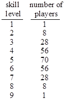
A more fundamental approach would be to model the underlying process. For example, suppose there are 256 ranked players in the world, with skill levels ranging from 1 to 9 distributed binomially as follows

Of course, "skill" might be a matrix rather than a scalar, and you could get into all sorts of interesting interactions (scissors cuts paper, paper wraps stone, stone breaks scissors, etc), but let's just assume that "skill" in this game can be modeled by a simple scalar. 

Now we must also specify to what extent skill determines the outcome of a contest. If the game's outcome is largely determined by chance, then the world's most skillful player may only beat the least skillful player 60% of the time. One way of modeling this is to say that the probability of player P_m beating player P_n is

where s_j is the skill of player P_j and the constant k determines the importance of skill in this game. As k goes to 0 all the probabilities go to 0.5, meaning that the outcome of a game is only weakly determined by skill. If k is very large, then the more skillful player will almost always win.

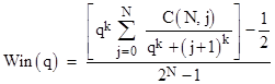
Now we have a simple but complete model for which we can compute the long-term win/loss records of each skill level. In general, for a league of 2^N players with binomially distributed skill levels and assuming a skill factor of k (and every player plays every other player equally often), the "winning percentage" of a player with skill level q is

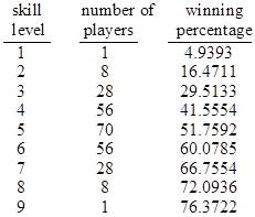
where C(N,j) is the binomial coefficient N!/((n-j)! j!). Taking N = 8 and k = 2, the winning percentages for each of the 9 skill levels are as shown below:

Of course, the weighted average of all these winning percentages is 50%. Also, since Win(q) is invertible, it follows that for any system of this general type the formula for predicting winners can be expressed in the form f(x)/[f(x) + f(y)].

Return to MathPages Main Menu