Feynman’s Ants

In his entertaining autobiography “Surely You’re Joking, Mr. Feynman” the physicist Richard Feynman described how he had studied the behavior of ants while he was in graduate school at Princeton and later when he was teaching at Caltech. The story can be taken as just an amusing illustration of Feynman’s eclectic curiosity and the lengths to which he would go to satisfy it, but it’s interesting that his analysis of the behavior of ants involves some of the same ideas that were central to his work in theoretical physics.

Feynman was awarded the Nobel prize in 1965 for his contributions to the theory of quantum electrodynamics. Much of this involved the development of a set of techniques for making quantum calculations and avoiding troublesome infinities (or, as he put it, “sweeping them under the rug”) by a process called re-normalization. Since there was (and still is not) any completely rigorous way of deriving this process, he was guided by some heuristic concepts (along with his own ingenuity). One of these heuristic concepts was the notion that the overall (complex) amplitude for a particle to move from A to B was proportional to the sum of the amplitudes of all possible paths between those two points. The phase of the contribution of each path was proportional to the length of the path. Now, we ordinarily think of particles (such as photons) as traveling in straight lines from A to B, but Feynman’s concept was that, in a sense, a particle follows all possible paths, and it just so happens that the lengths of nearly straight paths are not very sensitive to slight variations of the path, so they all have nearly identical lengths, meaning they have nearly the same phase, so their amplitudes add up. On the other hand, the lengths of the more convoluted paths are more sensitive to slight variations in the paths, so they have differing phases and tend to cancel out. The result is that the most probable path (by far) from A to B is the straight path. Compare this with Feynman’s description of his ant studies:

One question that I wondered about was why the ant trails look so straight and nice. The ants look as if they know what they're doing, as if they have a good sense of geometry. Yet the experiments that I did to try to demonstrate their sense of geometry didn't work. Many years later, when I was at Caltech … some ants came out around the bathtub… I put some sugar on the other end of the bathtub… The moment the ant found the sugar, I picked up a colored pencil  … and behind where the ant went I drew a line so I could tell where his trail was. The ant wandered a little bit wrong to get back to the hole, so the line was quite wiggly, unlike a typical ant trail.

When the next ant to find the sugar began to go back, I marked his trail with another color… he followed the first ant's return trail back, rather than his own incoming trail. (My theory is that when an ant has found some food, he leaves a much stronger trail than when he's just wandering around.) This second ant was in a great hurry and followed, pretty much, the original trail. But because he was going so fast he would go straight out, as if he were coasting, when the trail was wiggly. Often, as the ant was "coasting," he would find the trail again. Already it was apparent that the second ant's return was slightly straighter. With successive ants the same "improvement" of the trail by hurriedly and carelessly "following" it occurred. I followed eight or ten ants with my pencil until their trails became a neat line right along the bathtub.

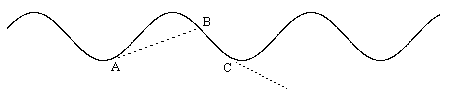
Admittedly the ant process of arriving at a straight path is not conceptually identical to the process of constructive and destructive interference, but there are strong similarities. The ultimate ant path turns out to be a result of multiple paths, with their mutual intersections converging on a straight line. The general idea presented by Feynman for why successive paths tend to become straighter is illustrated below.

The solid wavy line represents the first ant’s path. According to Feynman, the second ant follows the first path, but sometimes he “would go straight out, as if he were coasting”. By using the word “straight” here, Feynman is tacitly acknowledging that each individual ant actually does possess some innate propensity for “straightness”, presumably due to its own physical symmetries, and he is invoking this propensity in order to explain the asymptotic global straightness of their common trails. Sure enough, if an ant begins to “coast” at point A, and go “straight out”, it will re-encounter the original path at point B, and the new path is somewhat straighter than the original path. However, if the ant begins to “coast” at point C, he will never re-encounter the path, at least not without changing course and heading back toward the original path, in which case the resulting path is less straight than the original. So, the idea of “going straight, as if he were coasting” doesn’t by itself account for the progressively straighter paths. There must be more to it.

Feynman summarized the process he imagined by saying

It’s something like sketching: you draw a lousy line at first, then you go over it a few times and it makes a nice line after awhile.

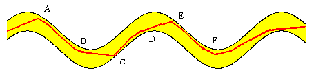
When we sketch in this manner, we are taking into view more than just the markings at the point of the pencil. We are looking at the surrounding markings, and averaging out the wiggles. If the ants are to do something similar, then either the trail markings must have some non-zero width, or the ants must be able to sense the presence of a trail from some non-zero distance away. In either case, we can represent the results in terms of point-like ants on scented trails with some non-zero width, as illustrated below.

In this case the rule for ant navigation could be to follow along the boundary of a trail as long as it is fairly straight (locally), but if it begins to curve, the ant may “coast along” in a straight line (staying always on the trail) until it hits another boundary, at which point it resumes following the boundary. This is shown by the red path in the figure above, and it does indeed result in a reduction in the amplitude of the deviations from an overall straight path. The red path would be the centerline of a new trail with some non-zero width, and the next ant would follow the same rule of navigation, resulting in a still straighter path. And so on.

Another aspect of Feynman’s physics that had a counterpart in his study of ants is his interest in the notion of particles and waves traveling backwards in time. His “absorber theory” made use of the advanced potential solutions of Maxwell’s equations, and his concept of particle interactions was largely time-symmetrical. In his popular book “QED” he wrote about the mediation of the electromagnetic force by photons:

I would like to point out something about photons being emitted and absorbed: if point 6 is later than point 5, we might say that the photon was emitted at 5 and absorbed at 6. If 6 is earlier than 5, we might prefer to say the photon was emitted at 6 and absorbed at 5, but we could just as well say that the photon is going backwards in time! However, we don't have to worry about which way in space-time the photon went; it's all included in the formula for P(5 to 6), and we say a photon was "exchanged." Isn't it beautiful how simple Nature is!

Similarly in his study of ants Feynman was interested in whether the paths were inherently directional. He wrote

I found out the trail wasn't directional. If I'd pick up an ant on a piece of paper, turn him around and around, and then put him back onto the trail, he wouldn't know that he was going the wrong way until he met another ant.  (Later, in Brazil, I noticed some leaf-cutting ants and tried the same experiment on them. They could tell, within a few steps, whether they were going toward the food or away from it—presumably from the trail, which might be a series of smells in a pattern: A, B, space, A, B, space, and so on.)

So we find in both his physics and his ant studies that Feynman was led to similar sets of questions, such as “How do straight paths arise from the motions of entities that have no innate sense of global straightness?”, and “Are the paths of entities inherently symmetrical in the forward and backward directions?” It’s hard to believe that he wasn’t conscious of these parallels when he wrote about his adventures with ants (in the chapter he entitled “Amateur Scientist”), and yet he never explicitly drew attention to the parallels. Admirable subtlety.

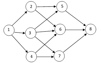
Speaking of Feynman’s “sum over all paths” approach to quantum mechanics, and parallels that we can find in more mundane contexts, I’m reminded of a little computational trick that I once saw in a industrial technical report on reliability analysis methods. The system to be analyzed was expressed in terms of a Markov model, consisting of a set of “states” with exponential transitions between states, such as shown in the diagram below.

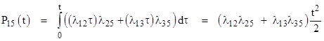
Each arrow represents a transition (of the system) from one state to another, and each of these transitions has an assigned exponential transition rate. (The similarity to Feynman diagrams is obvious.) Now, suppose the system begins at time t = 0 in State 1 with probability 1, and we wish to know the probability of the system being in State 8 at some later time t. Letting λ_ij denote the transition rate from state i to state j, we know that to the first non-zero order of approximation the probabilities of being in States 2, 3, and 4 at time t (small enough so that 1 – e^λt ≈ λt) are λ₁₂ t , λ₁₃ t , and λ₁₄ t  respectively. The lowest-order approximation of the probability of State 5 is given by the integral

Continuing on in this way, by direct integration, it’s clear that the lowest-order approximation (for small t) of the probability of transitioning from State 1 to another State is given by the sum over all possible paths of the product of the amplitudes (transition rates) along the paths. There is also a factor of t^k/k! for paths consisting of k transitions. The seven possible paths from State 1 to State 8 in the above model are

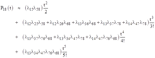
so the probability of transitioning from State 1 to State 8 by time t (for sufficiently small t) is given to the lowest non-zero order of approximation by

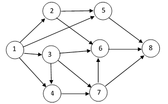
So, in the context of this simple reliability model, and to the lowest order of approximation, we can represent the transition probability as the sum of the products of the transition rates along every possible path. Needless to say, there are better ways of evaluating the probabilities of Markov models, but this crude technique is interesting because of its similarity, at least in form, to the sum of products of transition amplitudes in Feynman’s approach to quantum electrodynamics. On the other hand, there are some notable differences. First, the amplitudes in quantum electrodynamics are complex, with both a magnitude and a phase, whereas the transition rates in a reliability model are purely real and have no phase. Second, the reliability model we considered was rather specialized, in the sense that every path from one state to another consisted of the same number of individual transitions. For example, each path from State 1 to State 8 consisted of exactly three transitions. Because of this, the lowest order of approximation for the contribution of each path was of the same order as for each of the other paths. In general this need not be the case, as shown by the Markov model illustrated in the figure below.

The ten distinct paths from State 1 to State 8 in this model are

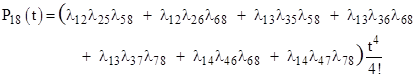
The path denoted by 158 proceeds from State 1 to State 8 in just two steps, whereas the path denoted by 124768 involves five steps. Using the calculation rule described above, adding together the products of the transition rates along each possible path, with a factor of t^k/k! applied to paths of length k, we get

However, the terms in t³, t⁴, and t⁵ are incomplete, because we have omitted the higher-order components of the full expressions for the lower-order paths. For example, the probability of path 158 actually contains terms in t³, t⁴, t⁵, and so on, but these are not included in the above summation. We have only included the lowest-order non-zero term for each path. Now, if all the λ values are small and of roughly the same size, we could argue that only the term in t² is significant, but we often cannot be sure the transition rates are all nearly the same size. It’s possible to choose the values of the λs in our example so that the only non-zero contribution to the probability is the path 134768 consisting of five transitions. Therefore we can’t necessarily neglect the 5^th degree term. But once we have recognized this, how can we justify omitting the 5^th degree contributions of the lower-order terms? The admittedly not very rigorous justification is that, assuming all the λs are orders of magnitude smaller than 1 (which is often the case in reliability models), each successive term in the contribution of a given path is orders of magnitude smaller than the preceding term. This implies that by including the lowest-order non-zero contribution of each path, we are assured of representing the most significant contributors to the probability – at least for the initial time period, i.e., for t sufficiently near zero.

The second Markov model above is more general than the first, in the sense that it allows two given states to be connected by paths with unequal numbers of transitions, but it is still not fully general, because it is free of closed loops. Once the system has left any given state it cannot return to that state. Loop-free systems are characterized by the fact that their eigenvalues are simply the diagonal elements of the transition matrix. This can be proven by noting that for such a system we can solve for the probability of the initial state independently, with eigenvalue equal to the diagonal element of the transition matrix, and then this serves as the forcing function in the simple first-order equation for the probability of any state whose only input is from the initial state. By direct integration the eigenvalue for the homogeneous part of the solution is again just the corresponding diagonal term in the transition matrix. We can then consolidate this state into the initial state and repeat the process, always solving for a state whose only input is from the (aggregated) initial state. This is guaranteed to work because in any loop-free system there is always a state of the first rank (i.e., a state that is just one transition away from the initial state) that can be reached by only one path, directly from the initial state. If this were not true, then every state of the first rank would have to be reachable by way of some other state of the first rank (possibly by way of some higher rank), and that other state would likewise have to be reachable by still another state of the first rank, and so on. Since there are only finitely many states, we must eventually either arrive at a closed loop, or else at a first-rank state that is not reachable by way of any other first (or higher) rank state, so it can only be reached from the zeroth rank state, i.e., the initial state.

There are, however, many applications in which closed loops do occur. For example, in reliability Markov models there are often repair transitions as well as failure transitions, such that if a component of the system fails, moving the system from one state to another, there is a repair transition by which the system can return to the un-failed state. So it’s important to consider models in which the system can undergo closed-loop transitions. Interestingly, regarding his study of ants, Feynman remarks that

I tried at one point to make the ants go around in a circle, but I didn’t have enough patience to set it up. I could see no reason, other than lack of patience, why it couldn’t be done.

Feynman also grappled with the concept of closed-loop paths in his work on quantum gravity. In his Lectures on Gravity he wrote

In the lowest order, the theory [of quantum gravity] is complete by this specification. All processes suitably represented by “tree” diagrams have no difficulties. The “tree” diagrams are those which contain neither bubbles nor closed loops… The name evidently refers to the fact that the branches of a tree never close back upon themselves… In higher orders, when we allow bubbles and loops in the diagrams, the theory is unsatisfactory in that it gets silly results… Some of the difficulties have to do with the lack of unitarity of some sums of diagrams… I suspect the theory is not renormalizable.

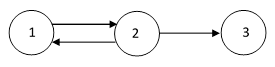
Likewise the existence of closed loops in a Markov model also presents some difficulty for the “sum over all paths” approach, because once closed loops are allowed, there can be infinitely many paths from one point to another. To illustrate, consider the simple model shown below.

The possible paths from State 1 to State 3 are now 123, 12123, 1212123, and so on. Each of these paths contains two more transitions than the previous path, and we could sum up the series of contributions using the “sum over all paths” rule, to give

but this is clearly wrong, because it changes the basic estimate in the wrong direction, i.e., it increases the probability of being in State 3 at any given time, whereas the transition path from State 2 back to State 1 actually decreases the rate of transitioning from State 1 to State 3. So the simplistic approach to the “sum over all paths” rule doesn’t work when we allow closed loops. However, it’s interesting to consider whether there might still be a sense in which the “sum over all paths” approach is valid.

If, instead of treating each system state and each transition individually, we consolidate them formally into a state vector P and a transition matrix M, then the system equations can be written succinctly as

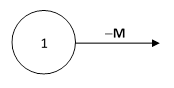
Since P₁ + P₂ + P₃ = 1, there are only two degrees of freedom, so we can take as our state vector just the two probabilities P₁, P₂. Now, the usual Markov model representation of this equation, if the matrix M and state vector P were scalars, would be an open loop

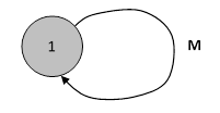
However, this doesn’t seem representative of a system of equations that may be closed loop, because this diagram suggests that probability continually flows out of the state, and never back into the state. For closed systems represented by (1) the probability components of the state vector may approach non-zero steady-state values, because there is flow back into the individual states. In a rough formalistic sense we might argue that a system equation like (1) can be placed in correspondence with a closed cloop model as shown below.

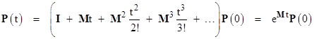
Admittedly this is not strictly a Markov model representation of (1), but it might be regarded as a meaningful notional representation. It’s interesting to examine the consequences of treating this model as if it was a Markov model. The paths from State 1 to itself consist of 1 (the null path), 11, 111, 1111, and so on. Using the original rule for expressing the probability of being in any given state as the sum of the products of the transition amplitudes for each possible path from the initial state to that given state, with each term multiplied by t^k/k!, we get

which of course is the solution of equation (1). Thus the individual “paths” correspond to terms in the series expansion of the solution. This applies to every linear first-order system of differential equations, regardless of whether the transitions encoded in M are open or closed loop. It’s interesting that this crudely motivated reasoning leads to a meaningful answer. Whether this kind of reasoning could be given a solid foundation is unclear.

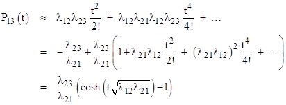
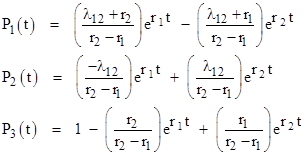
Another (slightly more rigorous) approach would be to express the individual state probabilities as scalar sums, just by expanding the individual solutions. In the above example the exact expressions for the probabilities of the three individual states are

where r₁ and r₂ denote the characteristic roots –α+β and –α–β with the symmetrical and anti-symmetrical parts

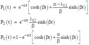
For non-negative real transition rates the quantity inside the square root is non-negative, since it can be written as (λ₁₂ - λ₂₃)² + (λ₁₂ + λ₂₁ + λ₂₃) λ₂₁, so α and β are real, and the individual state probabilities can be written in the form

The exponents of t in the series expressions for the hyperbolic sine and cosine functions increase by two in successive terms, so they can be seen (somewhat abstractly) as representing the cumulative contributions of the two-step loops between States 1 and 2.

But this reasoning is still not very rigorous. If we were trying to adhere rigorously to the heuristic concept of a “sum over all paths”, similar to Feynman’s approach to quantum electrodynamics, how might we proceed? We seek an expression (as a sum over all paths) for the probability of the system being in either State 1 or State 2 at time t. This quantity can be written as 1 – P₃(t), but we know the sum over paths method will not give this value directly, because each transition between the looping states (States 1 and 2) increases the overall sum of the system probability, which gives each of the states a probability that increases to infinity. We need to apply some re-normalization for the infinite loops in order to arrive at a finite result. Let us suppose that the normalizing factor equals the sum of the “symmetrical” part of the loop transitions, i.e., the part represented by a in the characteristic roots of the sub-system consisting of States 1 and 2 and the transition loop between them. This suggests the normalization factor

Therefore, we seek an expression of the form

Now we further suppose that β, the anti-symmetrical part of the characteristic roots, represents the geometric mean of the effective rates for transitioning from State 1 to State 2 and from State 2 to State 1, and that the former equals α. Then the latter equals

and β can also be written in the form

In these terms, the kth loop from State 1 back to itself contributes (βt)^2k/(2k)!, so we have

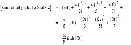
Likewise, since α is the effective rate for transitioning from State 1 to State 2, the sum of all paths (from the initial condition, which is State 1) to State 2 is

Thus our overall result is

from which we get

in agreement with the exact solution. So, by this indirect, heuristically-guided, ant-like meandering, with no rigorous justification for the steps, we arrive at the correct expression for the state probabilities.

Return to MathPages Main Menu