Markov Models Of Dual-Redundant Systems

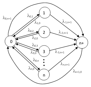
Many practical systems require numerous sub-functions to be performed in order to support the overall function, and they are designed to be dual-redundant on each sub-function. Failure of the first component of any particular sub-function is annunciated, and repaired at a suitable rate to preclude complete failure. In addition, there is a possibility of a single failure from the "full-up" condition leading to overall functional failure. This type of system with n sub-functions is often represented by a Markov model as shown below.

This model neglects the possibility that multiple sub-functions may be degraded at any given time. In other words, if one component of a certain sub-function fails, it is assumed that the next transition is either a repair back to the full-up state or else a failure of the other component of that same sub-function, resulting in total system failure. Strictly speaking, it’s possible that a component of some other sub-function might fail before either of those two transitions occurs, and this would place the system in a state with two of the sub-functions partially failed. However, this would affect the overall system failure rate only if both components of that second sub-function failed within the repair interval of the first sub-function, and both of those failures would need to occur prior to the failure of the second component of the first sub-function. Thus (for example) the transition rate λ_1,n+1 from state 1 to state n+1 should actually be augmented by the rate of failing both components of sub-function 2, consists not just of but also of (λ_2,n+1)² T where T is the repair interval. Similar terms would be needed to account for the other sub-functions. However, in many practical situations the repair intervals are small enough so that these second-order terms are negligible. This is why the simplified model shown above is often a useful representation of dual-redundant system reliability.

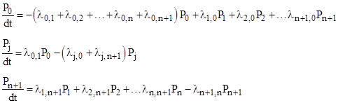
If we designate the “full up” state with the number 0, the n degraded states with the numbers 1 through n, and the final failure state with the number n+1, then the equations of the system can be written as

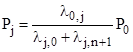
For the steady-state condition we have dP_j/dt = 0 for all j, so we can solve the central equations to give the values of P₁ through P_n as a function of P₀

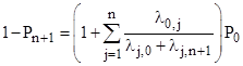
where λ_i,j signifies the rate of transition from state i to state j. Since the sum of all the state probabilities from P₀ to P_n+1 is 1, we have

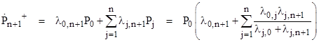
Also, the steady-state flow rate into State n+1 is

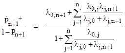
The exact failure rate for entering state n+1 is therefore

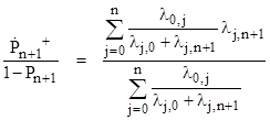
Naturally this rate is independent of λ_n+1,0, because the rate is, by definition, a measure of the propensity to enter a particular state for entities that are not presently in that state, which is clearly independent of the rate of leaving that state. Interestingly, if we define λ_j,j as infinite for each j, none of the state equations are affected, because the infinite "self-transition" flow P_jλ_j,j is both added to and subtracted from the jth equation, but this enables us to write the equation for the failure rate in the more unified form

This form emphasizes the fact that the overall rate for entering state n+1 is simply the weighted average of the individual transition rates λ_j,n+1 from each of the states 0, 1, 2, ..., n, with each rate weighted in proportion to the steady-state probability P_j of the respective state.

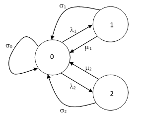
Since the time spent in the (n+1)th state is irrelevant to our result (because the reliability of the operational fleet does not depend on the length of time that inoperative systems are absent from the fleet while being repaired), we could simplify the analysis by deleting that state from the model, and point the total failure transitions directly to the full-up state. This is illustrated for a simple system with just two partial failure states in the figure below.

From the equations

we have the steady-state relations

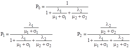
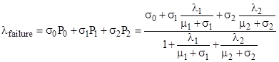
Substituting into the conservation equation P₀ + P₁ + P₂ = 1 allows us to easily solve for the steady-state probabilities

The total failure rate can then be computed as

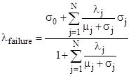
This immediately generalizes to give the formula for N partial-failure states as shown previously:

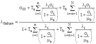
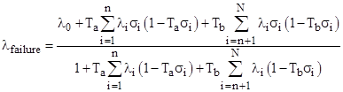
Suppose there are only two distinct repair rates, denoted by μ_a = 1/T_a and μ_b = 1/T_b, and we wish to express the overall rate as an explicit function of the repair times T_a and T_b. Let the indices 1 through n signify the states with repair rate μ_a, and the indices n+1 to N signify the states with repair rate μ_b. We can then re-write the above equation in the form

Assuming the failures rates are smaller than the repair rates, we can expand the fractions in powers of σ/μ, and to the first order we get

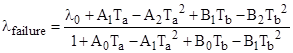
Collecting terms in T_a and T_b, we arrive at

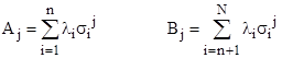
where the A_i and B_i coefficients are given by the summations

Return to MathPages Main Menu