Reliability With Mixed Periodic Repairs

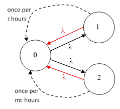
Consider a dual redundant system consisting of two components, each of which has a failure rate of λ. One of the components is checked and (if necessary) repaired periodically once every τ hours, and the other component is checked and repaired once every mτ hours, where m is some positive integer. The overall system is considered failed if both components are failed simultaneously, at which point the system is immediately repaired or replaced with a completely healthy system.

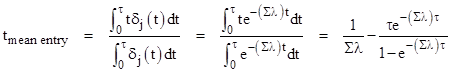
One simple way of evaluating the long term system failure rate is to approximate the repair transition for each state as continuous with constant rate equal to the reciprocal of the mean time to repair for that state. If the rate of entering the state is much less than the repair rate, then the system will enter the state at times that are almost uniformly distributed over the inspection interval, so the mean time to repair will be about half of the inspection interval. However, if the rate of entering the state is large compared with the repair rate, the mean time to repair will approach the full inspection interval. For a failure state j that is entered directly from the full-up state with a rate λ_j, the initial probability density for entering the failure state is roughly

where Σλ denotes the sum of the transition rates exiting the full-up state. Hence we can approximate the mean time of entry for systems that enter state j over an interval τ as

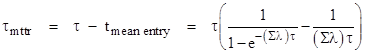
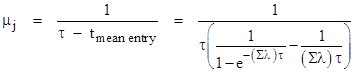
and so the mean time to repair for these systems is approximately

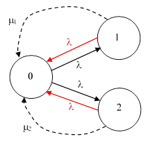
where τ is the inspection (and repair) interval. Naturally this is approximately τ/2 for sufficiently small values of τ. Using this formula, we can determine suitable values for the repair rates μ₁ and μ₂ of our dual redundant system, and the system can then be represented by the simple Markov model shown below.

The steady-state system equations are

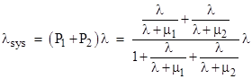
Solving these for P₁ and P₂, and inserting into the conservation equation P₀ + P₁ + P₂ = 1, we can then solve for P₀. From this we can express the system failure rate as

Does this simple approach accurately reflect the system response? We have substituted exponentially-distributed continuous repairs for periodic discrete repairs, so it would be of interest to evaluate the original system precisely, with no approximations, to allow us to compare the exact result with this approximate formula. The exact system is as shown in the figure below.

To solve for the exact long-term system failure rate, we first consider the time-dependent response of the original system, leaving out the discrete repairs. The system equations are

In terms of the sum S(t) = P₁(t) + P₂(t) and the difference D(t) = P₁(t) – P₂(t), these equations can be separated and written in the equivalent form

These are the governing equations in between discrete repairs. Thus during the period following the jth repair of State 1 we have

Our strategy is to begin with S_j(0) = D_j(0) = 0, and evaluate the results for m consecutive intervals of duration τ, and between each interval we will move all the accumulated probability from State 1 to State 0. The system failure rate is λS, and the average of the average rates for all m intervals represents our overall system failure rate.

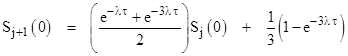
Noting that P₁ = (S+D)/2 and P₂ = (S−D)/2, we can say that the values of S and D at the end of one interval are related to the values at the start of the next (after P₁ has been set to zero while P₂ is held constant) according to the formulas

The left hand relation signifies that S_j(0) = −D_j(0) for all j. Making this substitution in the right hand relation, and also replacing D_j(τ) with D_j(0)e^−λτ, we get

Now we can substitute for S_j(τ) from the previous expression for S_j(t) at t = τ, to give the recurrence relation for the values of S at the start of each interval

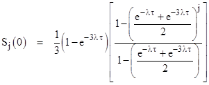
In general, given a linear recurrence of the form s_j+1 = As_j + B with the initial condition s₀ = 0, it’s easy to show that s_j = B(1−A^j)/(1−A). Therefore, we can express the value of S at the start of the jth interval in closed form as

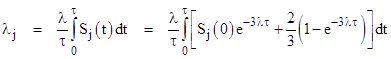
Furthermore, we know the average rate over the jth interval is

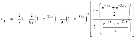
Carrying out the integration and inserting the previous expression for S_j(0), we get an explicit expression for the average system failure rate during the jth interval

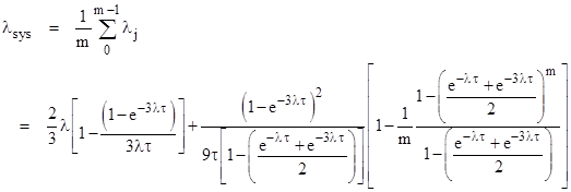
The average system failure rate over all m intervals is 1/m times the sum of the individual average rates. Only one of the terms in the expression for λ_j involves j, so the other terms all appear unchanged in the overall failure rate. For the remaining term, we can sum the geometric series and divide by m to give the final result

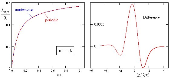
We can compare this with the ordinary Markov model approximation with continuous repair transitions discussed previously, making use of the estimated mean times to repair for determining the repair transition rates. The figure below shows the results for the case m = 10, i.e., the inspection interval for state 2 is ten times the inspection interval τ for state 1. The left hand figure shows the system failure rates for the two methods, and the right hand figure shows the difference between them.

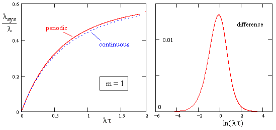
Clearly the agreement is very close for this case, but interestingly the agreement is not nearly as good if we consider the symmetrical case, i.e., with m = 1, signifying that both components have the same inspection interval. A comparison for the two methods in this case is shown below.

This shows that the overall system failure rate is appreciably greater with periodic repairs than with continuous repairs with (approximately) the same mean times to repair. Recall that the continuous repair model uses, for the jth state, a repair transition rate equal to the reciprocal of the estimated mean time to repair for a system entering that state, i.e.,

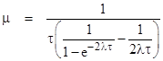
where τ is the duration of the inspection interval for the jth state and Σλ is the sum of the transition rates exiting the upstream state. In our case we have Σλ = 2λ, since there are two transitions exiting the full-up state, each with rate λ. Also, in the symmetrical case m = 1, the inspection intervals are τ for both states. Therefore, inserting the rate

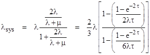
into the steady-state solution for the symmetrical Markov model with continuous repairs, we get the approximation

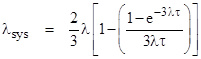
We can compare this with the exact periodic solution, which in the symmetrical case m = 1 reduces to

This result can also be derived by direct integration (as shown in another note), and we see that it does indeed differ from the prediction for continuous repairs. However, if we took Σλ equal to 3λ instead of 2λ, the Markov model with continuous repairs would give exactly the same system failure rate as the system with periodic repairs. This corresponds to increasing slightly the mean time spent by the system in each of the partial failure states. Nevertheless, the setting Σλ equal to 2λ definitely gives a better fit in the asymmetric cases, so no single value is optimum for all cases. Presumably the system failure rate with periodic repairs is greater than the rate with continuous repairs (with the same mean repair times) due to the lack of statistical independence between the two component failures with synchronized inspections. If the periodic inspections were staggered, we would expect the results to more closely match the continuous repair model with Σλ = 2λ. Still, it’s remarkable that, in the symmetrical case, this non-independence effect in the periodic model is exactly reproduced by setting Σλ = 3λ.

Return to MathPages Main Menu