|
Recurrence Relations for Ordinary Differential Equations |
|
|
|
Newton's identities can be used to compute the coefficients of multi-step recurrence formulae for simulating the solutions of ordinary linear differential equations of high order. This approach gives the exact root-matched recurrence formula without having to determine the complex roots of the characteristic polynomials. |
|
|
|
1.0 Introduction |
|
|
|
Let x(t) and y(t) denote continuous functions of time related according to the Nth order differential equation |
|
|
|
|
|
|
|
where the coefficients ak and bk are constants. Simple linear relationships of this form are widely used in numerical simulations of heat transfer, chemical reactions, fluid flows, mechanical dynamics, Markov processes, etc. [1] (Relationships of this form are also used in signal filtering and control-system compensation, but in those applications the frequency response is usually emphasized over the exact time-domain response.) A variety of methods (cf [2,3]) have been used to numerically generate the solutions y(t) of such equations for arbitrary forcing functions x(t). In the digital environment equation (1) is often simulated by means of a multi-step linear recurrence relation of the form |
|
|
|
|
|
|
|
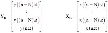
where Xn and Yn are the column vectors |
|
|
|
|
|
|
|
for some constant Δt (called the step-size of the simulation), and g and h are constant row vectors |
|
|
|
|
|
|
|
Given the coefficients ak and bk of (1), our objective is to compute, as quickly and efficiently as possible, the components of h and g. |
|
|
|
It
is well known [4] that if the recurrence is required to match the exact
homogeneous response for y(t) when x(t) is constantly zero, then the
components of h must be proportional to the elementary symmetric
functions [8] (with alternating signs) of the quantities |
|
|
|
2.0 Determining the Root Matched Recurrence |
|
|
|
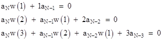
For any integer k, let w(k) denote the sum of the kth powers of the roots α1,α2,..,αN. Clearly, w(0) = N. Using Newton's Identities [8,9] the values of w(k) for k = 1,2,... are given by |
|
|
|
|
|
|
|
for k < N, and the recurrence |
|
|
|
|
|
|
|
for
all k ≥ N. Now let E(k) denote the sum of the kth powers of the values
of |
|
|
|
|
|
|
|
Letting
σk denote (–1)k times the kth elementary
symmetric function of the quantities |
|
|
|
|
|
|
|
The precision of these computations, including the convergence of (3), can be checked by verifying the equality |
|
|
|
|
|
|
|
The general recurrence for the homogeneous equation in y(t) can now be expressed as: |
|
|
|
|
|
|
|
where SA is the row vector |
|
|
|
|
|
|
|
Figure 1 presents an implementation of the preceding algorithm in BASIC. The inputs to this program are the order N, the step-size Δt, and the coefficients a0, a1 .., aN. The program computes the values of σ0, σ1,..,σN. The parameter "sumto" determines the number of terms to be evaluated in the summation (3). |
|
|
|
By entering the coefficients bk in place of ak into the preceding algorithm we can determine the recurrence for the homogeneous equation in x(t) |
|
|
|
|
|
|
|
We can then combine the two sides of the recurrence by applying the appropriate scale factors, which are easily deduced from steady-state conditions. The result is |
|
|
|
|
|
|
|
where ΣSA and ΣSB denote the sums of the components of SA and SB respectively. |
|
|
|
3.0 Equilateral Recurrences |
|
|
|
If bN = 0 then the characteristic polynomial of the right side of (1) has fewer than N roots. In this case the recurrence (4) would involve fewer "past values" of x(t) than of y(t). Note that the coefficients of xn in (4) were uniquely determined by the requirement that x(t) conform to the true homogeneous behavior when y(t) is constantly zero. However, in practice x(t) is an arbitrary forcing function so we are not really concerned with reproducing the homogeneous "response" of x(t). Instead, we are trying to reconstruct the function x(t) from the discrete samples. Thus it is often considered more appropriate to make use of as many past values of x(t) as is computationally convenient. This typically leads to recurrences that use the same number of past values of x(t) as of y(t), i.e., equilateral recurrences. The usual approach in signal processing is to augment the roots of the right-hand characteristic polynomial of (1) with fictitious roots of the form ±pi, and then proceed as before [10]. The effect is to add roots equaling –1 to the characteristic polynomial of the recurrence, which essentially mimics bi-linear substitution. |
|
|
|
The rationale for the "method of fictitious roots" just described is based on the frequency response characteristics. In the time domain it is often more appropriate to convert (1) into an equilateral equation by a simple change of variables. If we define the variable z(t) such that y = λ(x+z) for some constant λ, then (1) can be written |
|
|
|
|
|
|
|
For any choice of λ not equal to 0, (bN/aN), or (b0/a0), this equation is equilateral, so we can apply the method of (4) to give the recurrence |
|
|
|
|
|
|
|
where gλ is based on the coefficients of the right hand side of (5). Reverting back to the y(t) variable gives |
|
|
|
|
|
|
|
For large values of λ the vector λ(gλ + h) is quite insensitive to changes in λ, and it converges in the limit as |λ| → ∞. In practice, any λ greater than about 10 times the largest bi will give very nearly the limiting vector. This "change-of-variables method" enables us to determine equilateral recurrences for non-equilateral differential equations without resorting to fictitious roots. |
|
|
|
4.0 The Expected Value Method |
|
|
|
For comparison we briefly describe a method that explicitly treats x(t) as an independent variable and y(t) as a dependent variable. From this point of view it can be argued that the expected value of x(t) based on the N+1 most recent samples is given by the Nth degree polynomial that passes through those samples. Although the method is a straight-forward application of polynomial curve fitting, no explicit formulation of the general Nth-order recurrence formula appears in the literature, so a brief description is given below. |
|
|
|
As in our previous recurrence formulas, we require that the homogeneous response of y(t) be matched exactly, so we use the algorithm shown in Figure 1 to determine SA. Combining this with the particular solution based on the Nth order polynomial curve fit of x(t) leads directly to the total recurrence |
|
|
|
|
|
|
|
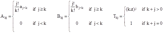
where A, B, and T are square matrices such that the elements in the jth columns of the kth rows (where j,k range from 0 to N) are given by |
|
|
|
|
|
|
|
This method gives, arguably, the best possible reconstruction of arbitrary forcing functions x(t), although the matrix inversions make it somewhat laborious when applied to high order equations. |
|
|
|
5.0 Examples |
|
|
|
To illustrate the basic algorithm for determining the root-matched recurrence relation for a homogeneous equation, consider the differential equation |
|
|
|
|
|
|
|
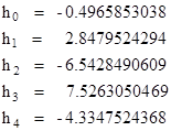
To simplify the recurrence expressions we will denote y(nΔt) by yn. Taking a time interval of Δt = 0.1, the algorithm described in Section 2 gives the following recurrence formula for yn |
|
|
|
|
|
|
|
where |
|
|
|
|
|
(Notice that we've scaled the coefficients to make h5 equal to 1.) The accuracy of this recurrence can be illustrated by noting that (6) has the characteristic roots –1, –2+i, –2–i, –1+i, and –1–i, so one particular analytical solution has the simple form |
|
|
|
|
|
|
|
Taking y0 through y4 from (8) as initial values, it is easily verified that the recurrence (7) numerically reproduces the exact analytical values of y5, y6, y7 ... etc., very precisely. After 35 iterations of the recurrence formula (carried out to 10 significant decimal digits) the value of y40 differs from the analytical value by only 0.0000013, this discrepancy being due entirely to accumulated round-off error. In contrast, using the recurrence relation given by bilinear substitution, the error at y40 is 0.0013094. For larger step-sizes the error using bilinear substitution becomes progressively worse, whereas the root-matched recurrence method is equally applicable to any step-size. |
|
|
|
We chose a homogeneous equation with simple characteristic roots for the preceding example so that the recurrence values could be easily compared to the analytical solution. Also, the characteristic roots in the preceding example all have negative real parts, so the solutions are "stable". However, our interest is not limited to "stable" systems. For example, problems involving combustion and thermal "run-away" often lead to "unstable" systems. To illustrate the various methods discussed in this note as applied to one of these "unstable" systems, and to include "numerator dynamics" [1], consider the differential equation |
|
|
|
|
|
|
|
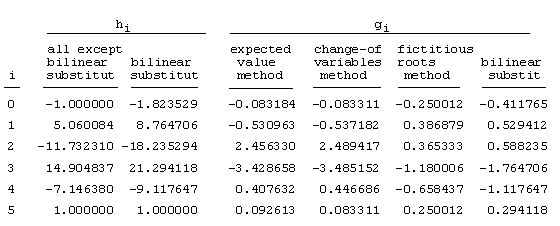
Taking a time interval of Δt = 1, the relation between x and y can be simulated using a linear recurrence of the form (2), where the components of h and g are as listed in the table below (normalized for h5 = 1). |
|
|
|
|
|
|
|
All the methods except Bilinear Substitution made use of the BASIC program in Figure 1 to determine the components of h and to assist in determining the components of g. Interestingly, the Change-of-Variables Method gives components of g that closely match those given by the Expected Value Method, even though the former makes no use of a 5th order curve fit of x(t). In contrast, the methods of fictitious roots and bilinear substitution give very different g vectors, and therefore will clearly yield significantly different values of y(t) in response to certain forcing functions x(t). |
|
|
|
6.0 Conclusions |
|
|
|
The technique described in this paper uses Newton's Identities to efficiently determine the root-matched recurrence relations for numerically simulating linear ordinary differential equations. The algorithm is simple to implement and can easily be incorporated into any numerical simulation program. The main benefit of the method is that it eliminates the need to determine the characteristic roots of the differential equation, which can be difficult for high order equations. This makes the method particularly useful in real-time applications that require frequent computation of recurrence relations corresponding to given continuous transfer functions. The recurrences given by this method (unlike bi-linear substitution) are valid for any step size Δt, provided only that the sampling period is small enough to adequately resolve the forcing function x(t). Also, the algorithm requires no special handling of characteristic equations with repeated roots, so it is applicable to any equation of the form (1). We have also shown how the "Change-of-Variables" method can be used to generate robust equilateral recurrences without resorting to fictitious roots. |
|
|
|
References |
|
1. E. O. Doebelin, System Dynamics, Modeling and Response, Charles E Merrill Publishing Company, 1972. |
|
2. V. Raman, "Explicit Multistep Methods In System Simulation", IEEE International Symposium on Circuits and Systems, 1989, vol 3, p 1792-1795. |
|
3. S. Sallam, W. Ameen, "Numerical Solution of General nth-Order Differential Equations Via Splines", Applied Numerical Mathematics, Vol 6, 1989/90, pp 225-238. |
|
4. A. L. Rabenstein, Elementary Differential Equations With Linear Algebra, Academic Press, 1970. |
|
5. J. M. Smith, Mathematical Modeling and Digital Simulation For Engineers and Scientists, 2nd Ed, John Wiley & Sons, 1987. |
|
6. T. Miyakodo, "Iterative methods for multiple zeros of a polynomial by clustering", Journal of Computational and Applied Mathematics, vol 28 (1989), p 315-326. |
|
7. V. J. Bucek, Control Systems, Continuous and Discrete, Prentice Hall, 1989. |
|
8. A. Clark, Elements of Abstract Algebra, Dover Publications, 1984. |
|
9. I. N. Herstein, Topics In Algebra, 2nd Ed, John Wiley & Sons, 1975. |
|
10. G. F. Franklin, J. David Powell, M. L. Workman, Digital Control of Dynamic Systems, 2nd Ed, Addison-Wesley, 1990. |
|
|