Complete Solutions of Linear Systems

A system of N first-order linear homogeneous differential equations with constant coefficient can be expressed in matrix form as

where P(t) is a column vector consisting of the N functions P₁(t), P₂(t)..., P_N(t), and M is the N ´ N coefficient matrix. Assuming the determinant of M is non-zero (meaning that the N equations are independent), and assuming we are given the initial values P(0), the complete solution of this system of equations can be expressed formally as

This can be used to compute the values of each function P_j(t) for any given time t, but it is sometimes useful to have explicit expressions for the individual functions P_j(t). To find these, first let f(r) = |M-ρI| be the characteristic polynomial of the system, with the roots ρ₁, ρ₂, ..., ρ_N. To account for duplicate roots, let n denote the number of distinct roots, and let m_j denote the multiplicity of the jth distinct root. Thus m₁ + m₂ + .. + m_n = N. Then each individual component of P(t) is of the form

Our objective is to determine the coefficients C_i,j,k explicitly in terms of M and P(0). We begin by noting that if we let P^(s)(t) = d^sP(t)/dt^s denote the s-th derivative of P with respect to t, then equation (1) immediately implies

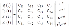
To express equations (3) in matrix form, it's convenient to place the C coefficients into an N ´ N matrix C, and place the factors of the form t^ke^ρt into a column vector E. To illustrate, for a system of degree N = 4 with n = 2 distinct roots, one of which has multiplicity m = 3, the general solution can be written as

Thus in general we can write P(t) = CE(t), and therefore

Letting [V₁, V₂, ..., V_N] denote the square matrix with columns V₁, V₂, ..., V_N, we can combine equations (4) and (5) to give

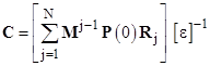
Hence the C matrix is given by

In these last two equations we omitted the argument (t) from the symbols for P(t) and E(t), with the understanding that they are all evaluated at the same t. Given the initial vector P(0), it is convenient to perform all the evaluations at t = 0. On this basis, each element of E⁽⁰⁾ is either 1 (for the first appearance of a distinct root) or 0 (for subsequent appearances), and the remaining columns E^(j) can be formed by a simple rule. In general, if the ith element of E⁽⁰⁾ is of the form e^ρt, then the corresponding row of the square matrix composed of the "E" columns is simply

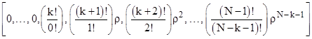
On the other hand, if there are repeated roots, some of the elements of E⁽⁰⁾ will be of the form t^ke^ρt, for which the corresponding row begins with k zeros, and then has the remaining terms indicated below

Naturally if k = 0 this reduces to the previous form. Letting [ε] denote the square matrix whose columns are the E^(j)(0) vectors, and making use of the orthogonal unit row vectors R₁ = [1,0,0,..], R₂ = [0,1,0,...], etc., we can write equation (6) more compactly as

and therefore the complete solution can be written explicitly in the form

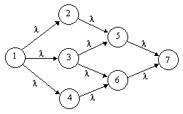
To illustrate this on a simple example, consider the simple monotonic Markov model shown below, where all the probability is initially in state 1.

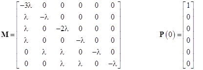
The system is conservative, so the sum of all the state probabilities is always 1, which implies that the seven system equations are not independent. Taking the equations for the states 1 through 6 as the independent equations of the system, we have P⁽¹⁾(t) = MP(t) where

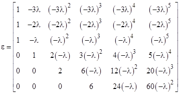
The six eigenvalues of the system, found by solving for the roots of the characteristic polynomial give by the determinant |M-ρI|, are

Thus we have three distinct roots, one of which has multiplicity four. From this we immediately have the matrix ε comprised of the E^(j)(0) column vectors

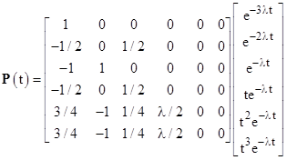
Substituting into equation (7) we get

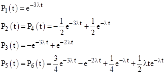
so we can write out the individual time-dependent probability functions explicitly as follows:

The time-dependent probability of state 7 is just the complement of these, so we have

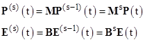
Incidentally, notice that equations (4) and (5) imply

so, if C is invertible, we have

If all the roots of the characteristic polynomial are distinct, this equation implies that C^-1MC is the diagonal matrix whose diagonal terms are the eigenvalues of the system. Thus the C matrix essentially just defines the conjugacy transformation that diagonalizes the system equations represented by M. (For a given matrix M there are N degrees of freedom in C, corresponding to the freedom to define the N components of the initial state vector P(0).) Another way of saying this is that P and E are, in a sense, formal duals of each other. Letting B denote N ´ N matrix C^–1MC, we can write

where the matrices M and B are conjugates, i.e., we have CB = MC. Now, still assuming that C is invertible, it follows that the (E,B) system is just a diagonalized version of the (P,M) system, with the same eigenvalues. If we were to apply the same analysis as above to this diagonalized system, the resulting "C" matrix would simply be the identity matrix I.

Of course, in the example worked above, the C matrix is not invertible. This signifies the fact that the components of P(t) do not constitute a complete basis, because the solution for the given initial values happens to be degenerate, and doesn't involve any multiples of t²e^ρt or t³e^ρt.

Return to MathPages Main Menu