Markov Models With Variable Transition Rates

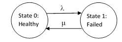
Perhaps the simplest Markov model in reliability analysis represents a single component with two possible states, healthy and failed. If the failures are exponentially distributed in time, with a constant rate λ, and if the failed unit is repaired or replaced at a constant rate μ, we can represent the model as shown below.

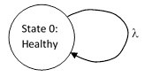
If we stipulate that failed units are repaired immediately, then the repair rate μ is infinite, and the probability of being in State 1 is zero. In this case we can eliminate that state, and depict the system as shown below.

Since the total probability is 1, we see that P₀(t) = 1 identically, and the failure rate is simply λP₀(t) = λ. Thus, even though this is a stationary system in the sense that nothing changes with time, it is still dynamic in the sense that it has a definite non-zero rate of exiting and re-entering the state.

The original defining characteristic of a Markov model was that the future state of the system depended only on the present state, not on the history of the system. Of course, to some extent this “Markovian property” is ambiguous, because we can define the “history” of a system as a state variable. For example, we might define the age of a component as a state variable, in which case a model with transition rates that depend on the age of the component would possess the Markovian property, whereas the very same model would be considered non-Markovian is we deny that the system age is a state variable. In many cases, what we regard as a function of time or age is really a function of the physical configuration on some higher level of resolution. For example, a wear-our characteristic is sometimes considered to be simply a function of “age”, but it could also be defined as a function of the more detailed aspects of the physical configuration – aspects that just happen to correlated with the time-since-new.

To make the definition of the Markovian property less ambiguous, it is sometimes identified with the condition that all transition rates are constants. It follows that such systems are homogeneous in time, which is to say, the origin t = 0 of the time coordinate can be located at any instant, and the system equations remain valid. On the other hand, if a transition rate is a non-constant function of time, the system equations will be valid only for one particular choice of the origin t = 0, which must be the instant when all the components of a system are new, so that the time parameter t can be identified with the age of the components. We may dis-allow the use of the time parameter itself as a state variable, but it is still possible to contrive homogeneous Markov models that simulate systems with variable transition rates.

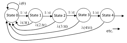
Consider again the simple system described above, but now instead of a constant failure rate λ, suppose the failure rate is an arbitrary function λ(t) of time, i.e., the age of the component from when it was new or most recently overhauled. Now, we cannot simply represent this model as depicted previously, because State zero will contain a mixture of systems of different ages, depending on how recently each system exited and returned to this State. The single binary state variable (healthy or failed) is not sufficient to fully determine the causal state of the system. To remedy this, suppose we split up the “healthy” state into a sequence of several states, and allow the system to transition from one to the next at rates that ensure uniform progression. From any one of these healthy states, the system can fail and be replaced or refurbished immediately back to the initial healthy state, as shown below.

We have assigned a rate of 1/Δt to each transition rate from one state to the next, so that the mean time from one state to the next is Δt. Then we assign a constant failure rate of λ(nΔt) to the nth state in this sequence. This arrangement simulates the variation in the failure rate as a function of the elapsed time since the system was most recently in State 0. The steady-state equation of the nth state (except for State 0) is

Thus we can define the ratios q_n of the probabilities of consecutive state

Consistent with this, we will define q₀ = 1. Now we can express the individual probabilities as

and so on. The sum of all the probabilities is 1, so we have

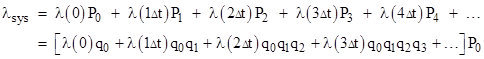
The system failure rate is

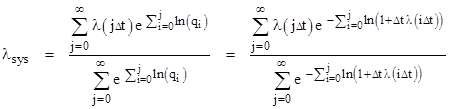
Combining these expressions gives the system failure rate entirely in terms of the individual component failure rates for all the “ages” from t = 0 to infinity:

This can be written in the form

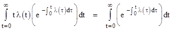
In view of the series expansion ln(1+x) = x – x²/2 + x³/3 - … we see that, in the limit as Δt goes to the infinitesimal dt, the natural logs go to dt λ(i dt). To avoid confusion we will let τ denote the time parameter appearing in the inner summation, and t will denote the time parameter in the outer summation. Then we have τ = i dτ and t = j dt, so if we multiply the numerator and denominator by dt, the above equation can be written in terms of continuous integrations as

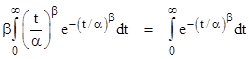
In order for a function λ(τ) to be a rate function, its integral from 0 to t must increase monotonically to infinity as t increases. In that case, the numerator of the above expression (which we recognize as simply the integral of the density function corresponding to the rate λ) equals 1, so we have

It’s easy to see that if λ(t) is constant, this expression reduces to λ, as expected. For a slightly less trivial example, suppose the failure rate varies as a Weibull distribution

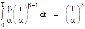
which has the integral

Inserting this into the equation for the system failure rate gives

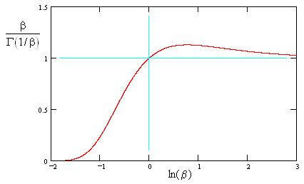
Of course, the case β = 1 is simply a constant rate, and this formula gives λ_sys = 1/α. In general, for arbitrary values of β, the integral can be evaluated in terms of the gamma function, and we find that the “closed loop” failure rate of a system with immediate repair and a Weibull distribution with parameters α,β is

A plot of the right hand factor is shown below.

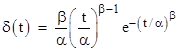
This shows that the recurrence rate stays fairly close to 1/α for β > 1, but drops toward zero for β < 1. Of course, the same result can be found by simply evaluating the mean time to failure for the Weibull distribution. As described in the note on Weibull analysis, the density distribution corresponding to the hazard rate (3) is easily shown to be

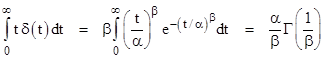
The mean time to failure is therefore

and the reciprocal of this is the mean recurrence rate, in agreement with the previous result expressed by equation (4). Comparing these two expressions, we see that

More generally, for any valid rate function λ(t), we have

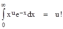
In a sense this is a generalization of the fact that 0! = 1!, which appears in the identity

Since the recurrence rate can be determined directly by integrating t δ(t) in these simple cases, there is no practical advantage to using the Markov model, except as an alternate means of deriving the density function. However, this approach can be used to introduce time-dependent transition rates into more general Markov models, whose density distributions are less obvious.

Return to MathPages Main Menu