Failure Rates, MTBFs, and All That

Suppose we're given a batch of 1000 widgets, and each functioning widget has a probability of 0.1 of failing on any given day, regardless of how many days it has already been functioning. This suggests that about 100 widgets are likely to fail on the first day, leaving us with 900 functioning widgets. On the second day we would again expect to lose about 0.1 of our functioning widgets, which represents 90 widgets, leaving us with 810. On the third day we would expect about 81 widgets to fail, and so on. Clearly this is an exponential decay, where each day we lose 0.1 of the remaining functional units. In a situation like this we can say that widgets have a constant failure rate (in this case, 0.1), which results in an exponential failure distribution. The "density function" for a continuous exponential distribution has the form

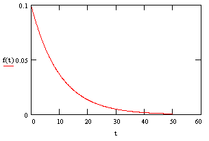
where λ is the rate. For example, the density function for our widgets is (0.1)exp(–t/10), which is plotted below:

Notice that by assuming the probability of failure for a functioning widget on any given day is independent of how long it has already been functioning we are assuming that widgets don't "wear-out" (nor do they improve) over time. This characteristic is sometimes called "lack of memory", and it's fairly accurate for many kinds of electronic devices with essentially random failure modes. However, in each application it's important to evaluate whether the devices in question really do have constant failure rates. If they don't, then use of the exponential distribution may be misleading.

Assuming our widgets have an exponential failure density as defined by (1), the probability that a given widget will fail between t = t₀ and t = t₁ is just the integral of f(t) over that interval. Thus, we have

Of course, if t₀ equals 0 the first term is simply 1, and we have the cumulative failure distribution

which is the probability that a functioning widget will fail at any time during the next t units of time. By the way, for any failure distribution (not just the exponential distribution), the "rate" at any time t is defined as

In other words, the "failure rate" is defined as the rate of change of the cumulative failure probability divided by the probability that the unit will not already be failed at time t. Notice that for the exponential distribution we have

so the rate is simply the constant λ. It might also be worth mentioning that the function e^x has the power series representation

so if the product λt is much smaller than 1 we have approximately e^x ≈ 1 + x, which when substituted into (2) gives a rough approximation for the cumulative failure probability F(t) ≈ λt.

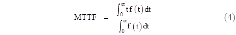
Now, we might ask what is the mean time to fail for a device with an arbitrary failure density f(t)? We just need to take the weighted average of all time values from zero to infinity, weighted according to the density. Thus the mean time to fail is

Of course, the denominator will ordinarily be 1, because the device has a cumulative probability of 1 of failing some time from 0 to infinity. Thus it is a characteristic of probability density functions that the integrals from 0 to infinity are 1. As a result, the mean time to fail can usually be expressed as

If we substitute the exponential density f(t) = λe^-λt into this equation and evaluate the integral, we get MTTF = 1/λ. Thus the mean time to fail for an exponential system is the inverse of the rate.

Now let's try something a little more interesting. Suppose we manufacture a batch of dual-redundant widgets, hoping to improve their reliability in service. A dual-widget is said to be failed only when both sub-widgets have failed. What is the failure density for a dual-widget? This can be derived in several different ways, but one simple way is to realize that the probability of both sub-widgets being failed by time t is

so this is the cumulative failure distribution F(t) for dual-widgets. From this we can immediately infer the density distribution f(t), which is simply the derivative of F(t) (recalling that F(t) is the integral of f(t)), so we have

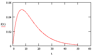
Notice that this is not a pure exponential distribution anymore (unlike the distribution for failures of a single widget). A plot of this density is shown below:

Remember that the failure density for the simplex widgets is a maximum at t = 0, whereas it is zero for a dual-widget. It then rises to a maximum and falls off. What is the mean time for a dual-widget to fail? As always, we get that by evaluating equation (5) above, but now we use our new dual-widget density function. Evaluating the integral gives MTTF = (3/2)(1/λ).

It sometimes strikes people as counter-intuitive that the early failure probability of a dual-redundant system is so low, and yet the MTTF is only increased by a factor of 3/2, but it's obvious from the plot of the dual-widget density f(t) that although it does extremely well for the early time period, it eventually rises above the simplex widget density. This stands to reason, because we're very unlikely to have them both components of a dual-widget fail at an early point, but on the other hand they each component still has an individual MTTF of 1/λ, so they it isn't likely that either of them will survive far past their mean life.

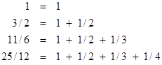
By the way, by this same approach we can determine that a triplex-widget would have a mean time to failure of (11/6)(1/λ), and a quad-widget would have an MTTF of (25/12)(1/λ). The leading factors are just the partial sums of the harmonic series, i.e.,

and so on. For more on this, see the note on Infinite Parallel Redundancy.

Return to MathPages Main Menu