Series Solution for Relativistic Orbits

Solving the field equations of general relativity for the orbit of a small test particle in Schwarzschild spacetime leads to the non-linear differential equation

where m is a measure of the mass of the gravitating body, h is a measure of the angular momentum, and u = 1/r. The parameters m and h are both normalized to have units of length. The second derivative of u in the above equation is with respect to the angular position θ in the orbit. The second term on the right side is what distinguishes this equation from the Newtonian equation of motion. An approximate solution of (1) for planetary orbits is given in Anomalous Precesion, but it’s also interesting to consider the power-series solution to this equation. Let u be represented by the infinite series

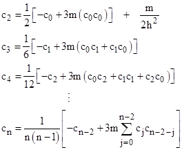
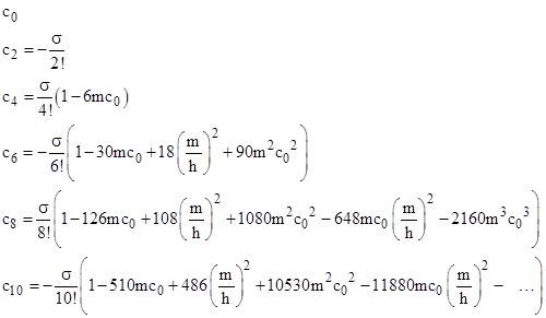
where c₀, c₁, … are real constants. Inserting into (1) and collecting terms by powers of θ, and setting each coefficient to zero, we get the following conditions on the coefficients:

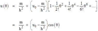
If the term of (1) involving u² was absent, the convolutions in the above equations would also be absent, and we would have simply c_n = −c_n−2 / (n(n−1)). This is the Newtonian case, and with the initial conditions c₀ = u₀ and c₁ = 0 we have

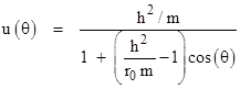
Thus the bound Newtonian orbits satisfy the equation

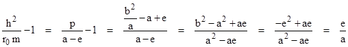
which is the equation of a conic section with the gravitating body at one focus. The ratio p = h²/m is the semi-latus rectum, and r₀ is the perihelion radius. Letting a and b denote the major and minor radii and e the linear eccentricity of the ellipse, we have the elementary relations e² = a² – b² , p = b²/a, and r₀ = a – e, so the quantity in parentheses in the above equation can be written as

Thus the quantity in parentheses is the numerical eccentricity ε = e/a. The orbit is an ellipse, a hyperbola, or a parabola respectively depending on whether |ε| is less than, greater than, or equal to 1.

To account for the relativistic correction term involving u² in equation (1) we must include the convolution terms in the series coefficients. We again find that, with the initial condition c₁ = 0, all the subsequent coefficients of odd powers of θ are also zero, so u(θ) is an even function (meaning it is the same in both directions of θ).

For the planet Mercury the orbital eccentricity is e = 0.026, the semi-major axis is a = (5.79)10⁷ km, and the normalized mass of the gravitating body (the sun) is m = 1.475 km. From these we can compute the perihelion distance r₀ = (1−e)a = (4.59)10⁷ km, and we also have

Setting c₀ = 1/r₀, we can evaluate the power series coefficients of u(θ) to give

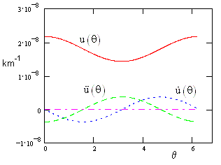
and so on.  Based on the first 60 terms (which is 30 non-zero terms, since all the odd-ordered terms are zero), the function u(θ) and its derivatives are plotted below.

The first derivative is zero at each perihelion and apihelion, and the first apihelion occurs at θ = 3.14159290423…, which exceeds π by (2.506)10⁻⁷ radians. Since u(θ) is an even function, we know the increment is the same for the apihelion near –π, so the total precession per revolution is twice this amount, which is (5.012)10⁻⁷ radians per revolution, equal to 0.1034 arc seconds per revolution. Mercury completes 414 revolutions per century, so it’s relativistic precession is 42.9 arc seconds per centuy, in close agreement with the observational value.

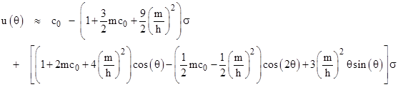
Algebraically the first several coefficients of the power series of u(θ) are

where

The first order of approximation beyond the Newtonian solution is given by the terms in mc₀ and (m/h)². The coefficients of the former are 6, 30, 126, 510, …, which can be expressed as 2(4ⁿ – 1) for n = 1, 2, 3, …, and the coefficients of the latter are 18, 108, 486, …, which can be expressed as 8(4ⁿ – 1) – 6n for n = 1, 2, 3, …  Making these substitutions and consolidating the resulting series into trigonometric functions, we get the result

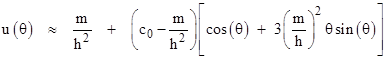
Naturally we still have u(0) = c₀., since the contributions of the other terms cancel out at this special value. Now, since c₀ and m/h² are many orders of magnitude smaller than 1 (for typical astronomical situations), the constant term is closely approximated by simply m/h². Also, the term involving cos(2θ) represents just a very slight periodic oscillation affecting the shape of the orbit, with no secular effect. Thus to determine the secular effects we can examine the close approximation

The quantity 3(m/h)²θ is very small for the first few revolutions, so for this part of the curve the quantity in the square brackets can be closely approximated by

Consequently the orbit precesses by 6π(m/h)² per revolution. The term involving θ sin(θ) appears naturally from the conditions on the power series coefficients, but it is often introduced simply as a trial solution, and/or justified as a resonance term. Of course, for sufficiently large angles θ, the approximation for u(θ) increases without limit, but m/h is so small that the above expressions are valid over many revolutions.

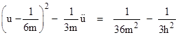
Incidentally, for some special cases we can find an exact closed-form solution to equation (1). Notice that (1) can be written in the form

In the special case when h² = 12m². the right hand side vanishes, and we have the equation

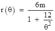
This has the exact solution y = 2/(mθ²), so we have

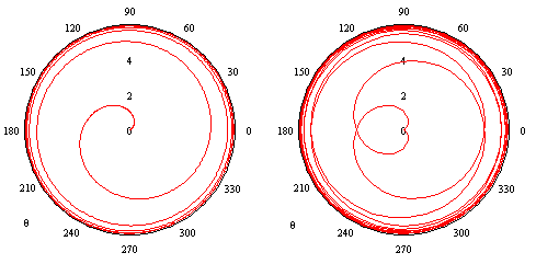
Hence the orbit spends infinitely much time arbitrarily close to a circular orbit at radius 6m for large negative values of θ, but then as θ approaches zero the orbit spirals down to the center of the field, as shown in the left-hand figure below.

Assuming it continues through the singularity as θ passes through zero, the orbit then spirals back up and re-converges on a circular orbit of radius 6m, as illustrated in the right-hand figure above.

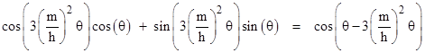
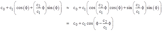
Incidentally, the relativistic contribution to a planet's orbital precession rate is often described as a "resonance" effect. Recall that the general solution of an ordinary linear differential equation contains a term proportional to e^λx for each root λ of the characteristic polynomial, and a resonance occurs when the characteristic polynomial has a repeated root, in which case the solution has a term proportional to xe^λx. If there is another repetition of the root it is represented by a term proportional to x²e^λx, and so on.  As a means of approximating the solution of the non-linear equation (6), many authors introduce a trial solution of the form c₀ + c₁cos(ϕ) + c₂ϕsin(ϕ), suggesting that the last term is to be regarded as a resonance, whose effect grows cumulatively over time because the factor ϕ is not periodic, and therefore eventually has observable effects over a large number of orbits, such as the 414 revolutions of Mercury per century.  Now, provided (c₂/c₁)ϕ is many orders of magnitude smaller than 1, we can indeed use the small-angle approximations sin(x) ~ x and cos(x) ~ 1 to write the solution as

where we’ve used the trigonometric identity cos(x)cos(y) + sin(x)sin(y) = cos(x−y). This yields the correct result, but the interpretation of it as a resonance effect is misleading, because the predominant cumulative effect of a resonant term proportional to ϕsin(ϕ) in the long run is not a precession of the ellipse, but rather an increase in the magnitude of the radial excursions of a component that is at an angle of π/2 relative to the original major axis. It just so happens that on the initial cycles this effect causes the overall perihelion to precess slightly, simply because the phase of the sine component is beginning to assert itself over the phase of the cosine component.  In other words, the apparent "precession" resulting from the ϕsin(ϕ) term on the initial cycles is really just a one-time phase shift corresponding to a secular increase in the radial amplitude, and does not actually represent a change in the frequency of the solution. It can be shown that a term involving ϕsin(ϕ) appears in the second-order power series expansion of the solution to equation (6), which explains why it is a useful curve-fitting function for small ϕ, but it does not represent a true resonance effect, as shown by the fact that the ultimate cumulative effect of this term is discarded when we apply the small-angle approximation to estimate the frequency shift.

Return to MathPages Main Menu