Hierarchical Repair and Quantum State Reduction

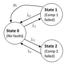
Consider a system consisting of two components with constant failure rates λ₁ and λ₂, and suppose the first component is repaired at the constant rate μ₁, and if both components are failed, the system is repaired (or replaced) immediately. In addition, the second component is periodically checked and (if necessary) repaired every T hours. The simple Markov model for this system is shown below, excluding any representation of the periodic inspection/repairs.

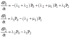
The fully-failed state is omitted, because that state contains no probability (since it is repaired immediately). The time-dependent state equations for this system are

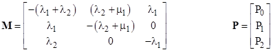
It’s convenient to express this set of equations in matrix notation as

where

Given any initial conditions P(t) at time t, the state probabilities at some later time t+T are given by

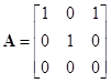
Now, at the initial time t = 0 we have P(0) = Transpose[1 0 0], and at the end of the first T-hour periodic inspection interval this formula gives the new state probabilities P(T). At this point we wish to inspect and repair any systems found in State 2 back to State 0. This can be accomplished by multiplying P(T) by re-distribution matrix A defined as

After the first interval T and carrying out the first inspection/repair, the state probabilities are P(T) = (Ae^MT)P(0), and after the second inspection/repair the state probabilities are P(2T) = (Ae^MT)² P(0), and so on. Therefore, after the nth inspection/repair, the state probabilities are

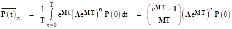
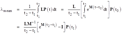
The average probabilities for the interval beginning at time nT is given by

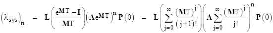
where I is the identity matrix. Notice that the numerator on the right hand side is divisible by MT, so it isn’t necessary to invert the M matrix. The system failure rate is λ₂P₁ + λ₁P₂, so if we define the row vector L = [ 0  λ₂  λ₁ ], the average system failure rate during the interval beginning at t = nT can be expressed as

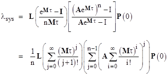
This example involved only one periodic inspection/repair interval, but the solution can be generalized to any number of distinct repair intervals. For example, suppose we have a system for which some of the components and inspected and (if failed) repaired every τ hours, whereas the remainder of the components are inspected/repaired only once every T = nτ hours. In other words, the longer interval is n times the smaller interval. For this system we have two “re-distribution matrices”, which we may call A and B. The first represents the repair of the τ-hour components, and the second represents the repair of all components, because everything is checked and repaired at the longer interval T. It can be shown (see below) that the average system failure rate is

We note that the B re-distribution matrix doesn’t appear in this expression, because B represents complete restoration of the system to the full-up state, so, beginning from the full-up state, we need only evaluate the system reliability over n of the t periods using the A matrix. At this point the B re-distribution would restore everything to the full-up state, so all subsequent iterations would be identical to the first.

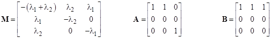
To illustrate, consider again the sample system discussed above, but suppose the first component did not contain continuous health monitoring (so μ₁ = 0), and instead it was maintained by a periodic inspection/repair every τ = 200 hours. As before, the second component is inspected and repaired periodically every T = 1000 hours. Thus we have n = 5, and the coefficient and re-distribution matrices are

Since the B matrix represents complete restoration of the system, we can use the preceding equation to evaluate the average system failure rate of one complete T-hour interval (which consists of five τ-hour intervals).

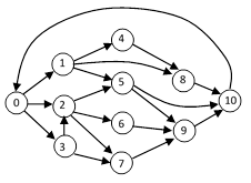
There is an interesting analogy between these reliability calculations (with periodic repairs) and quantum mechanics. In both cases the system’s state vector evolves according to linear equations, but this smooth evolution is interrupted by discrete inspections (and repairs) that have the effect of resolving some components of the state vector. To explain this analogy in detail, we will describe in more generality the method for evaluating the reliability of a system subjected to multiple periodic inspection/repair intervals. Consider the Markov model for a hypothetical system illustrated in the figure below.

Each node represents one of the observable states of the system, and in general we represent the state of the system at any time t by the state vector P(t), which we define as a column vector consisting of the probabilities of the system being in each of the states. Also, for each pair of states we have two rates, representing the rates at which the system would “decay” from one state to the other. (In general, the rates in the two directions may be different.) The time-dependent system equations are of the form

where M is a constant matrix consisting of all the transition rates. Given the state of the system at any time t₀, the state at any other time t is given by

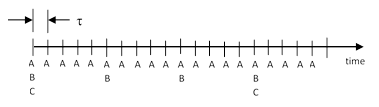
assuming the system is not disturbed from the outside during that interval of time. However, it is typical for systems to be periodically inspected (and repaired if necessary) at specified intervals of time. In fact, there may be a hierarchy of maintenance actions, such as cursory inspections every τ hours, and more complete inspections every nτ hours, and totally complete inspections every mnτ hours, as indicated schematically below.

The letters A, B, and C denote the three levels of inspections. Since the combination of the A, B, and C checks is complete, the system is placed in an identical “full-up” state once every mnτ hours. In the diagram above we have taken n = 5 and m = 3, meaning that a B check is performed once every five A checks, and a C check is performed once every three B checks. Each of these checks is analogous to a measurement or observation in quantum mechanics, and they have the effect of reducing the state vector, placing the system (or a subset of the system components) into a definite state, just as in quantum mechanics the state vector of a system becomes one of the eigenvectors after a measurement has been performed.

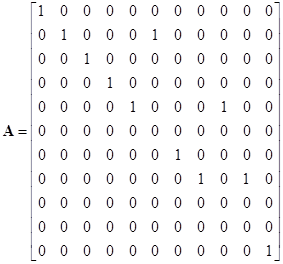
Suppose an A check consists of inspecting the system to determine if it is in one of the states 5, 8, or 9, and if it is found to be in one of those states, repairs are made so the system is placed in state 1, 4, or 7 respectively. (In other words, if the system is found in state 5, it is moved to state 1, and so on.) This operation can be represented by the matrix

Multiplying the state vector by this matrix leaves most of the state probabilities unchanged, but any probability of states 5, 8, and 9 is moved to the states 1, 4, and 7 respectively. Thus we know the probabilities of the states 5, 8, and 9 following this operation are precisely zero. Similarly the operations for the B and C checks can be represented by matrices. It’s worth noting that, although the coefficient matrix of the continuous time dependent solution is invertible (so they can be exercised forward or backward in time), these inspection matrices are generally not invertible.

Suppose state 10 is the “complete failure” state. The rate of entering that state at any given by the probabilities of states 5, 8, and 9 each multiplied by their respective rates for transitioning to state 10. Thus the system failure rate at any time t can be expressed as the dot product L∙P(t) where L is the row vector

Over any given interval of time, the mean system failure rate can therefore be determined by integrating the instantaneous rate as follows

where I is the identity matrix. If we let P_j denote the initial state vector for the jth time interval (between consecutive A checks), and note that each of these intervals is of length τ, we can say the average system failure rate for the jth interval is

Also, given the probability at the start of one interval, the probability at the end of that interval (prior to any inspections and repairs) is given by equation (1) as

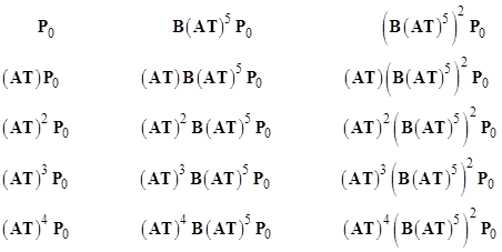
We’re now in a position to write down the average system failure rate for the entire sequence of hierarchical inspections and repairs. According to equation (2), it is just proportional to the average of the initial state vectors for the 15 intervals between C checks. These initial state vectors are given by multiplying the initial (“full up”) state vector P₀ by the cumulative transition matrices as listed below.

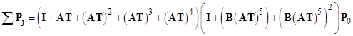
Letting I denote the identity matrix, we can factor the sum of these 15 initial state vectors as

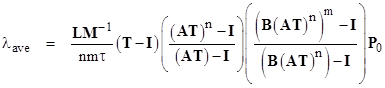
Summing each of the geometric series, multiplying by the rate factor from equation (2), and dividing by mn = 15 (to give the average), we get

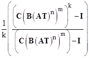
By the way, there is no ambiguity in the order of the divisions when expressing the geometric series in closed form, because all the implicit  multiplications are commutative. If there was another level in the inspection hierarchy, such as a D check occurring once every k checks at level C (and assuming D is complete and C is not), then the sequence of parenthetical terms in the above expression would be multiplied on the right by the factor

Similarly any number of hierarchies can be modeled by applying suitable factors in this way. The analogy with quantum mechanics is striking, even to the point of hierarchical observations, and the issues this raises with regard to the measurement problem. At what point can we say a measurement has taken place? If it has taken place at a low level, but not yet at a high level, can we (at the higher level) be sure the state vector has actually been reduced by the lower-level observation? It’s also interesting that the inspection operators are not invertible, so they represent irreversible processes, just as a measurement in quantum mechanics is irreversible. Of course, when dealing with reliability calculations we are restricted to real-valued probabilities rather than complex amplitudes, so there is no interference or quantum entanglement, but aside from this difference, the computational structure of Markov models in reliability is remarkably similar to the structure of quantum mechanics, especially in Heisenberg’s matrix formulation.

Return to MathPages Main Menu