Causality and the Wave Equation

Solutions of the standard wave equation can be expressed and interpreted in a variety of ways, leading to some interesting ideas about causality and temporal asymmetry in physical phenomena. Recall that, with just a single space coordinates (and one time coordinate) the ordinary wave equation for the scalar function ψ(x,t) is simply

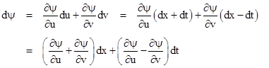
Usually the right hand side would be multiplied by 1/c², where c is the propagation speed, but for convenience we have chosen units of space and time so that c is unity. Now, for any function ψ(x,t) the total differential of ψ in terms of x and t is

Furthermore, if we define new coordinates u = x + t and v = x – t we have du = dx + dt and dv = dx – dt, and we can write this total differential as

Equating the coefficients of dx and dt in this last expression to those in the previous expression, we find the general relations between the differential operators

Thus the wave equation can be written in terms of the u,v coordinates as

Expanding the differential operators, canceling terms, and dividing by 4, this reduces to

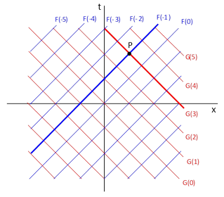
Since partial differentiation is commutative, this implies both of the relations

Thus the partial derivative of ψ with respect to v is independent of u, and the partial derivative with respect to u is independent of v. These are the necessary and sufficient conditions in order for a function ψ(u,v) to satisfy the wave equation. It follows that ψ is of the form F(v) + G(u) and so

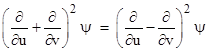
where F and G may be any functions whatsoever. Another way of deriving this result is to simply factor the differential operator representing the original wave equation as

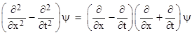
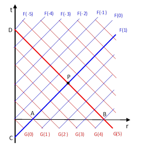
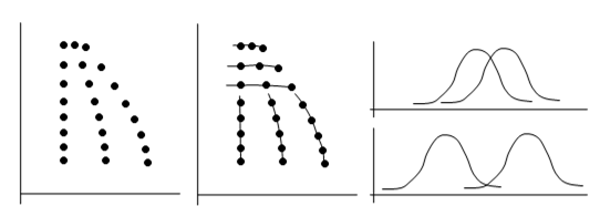
From this it follows immediately that ψ is of the form F(x - t) + G(x + t). It’s customary to regard these two terms as arbitrary waves propagating (at unit speed) in the positive and negative x directions respectively. This composition of ψ as a sum of two components is depicted in the figure below.

The point P has the (x,t) coordinates (1,2), and accordingly the field at this point is

Now, we may ask what causes the field to have this value at this point, and our answer seems to depend on how we have chosen to specify the constraints that determine the field. One way of doing this would be to specify the values of the F and G functions for every point on the x axis, corresponding to a time of t = 0. Thus, letting f(x,t) and g(x,t) denote the F and G components of the field at the point (x,t), we are “given” the values of f(x,0) and g(x,0) for all x. The field at the point P has the value f(–1,0) + g(3,0), and we could say these two components propagated from the locations x = –1 and x = 3 at time t = 0 to the point P at the time t = 2. This is the normal way of thinking about how effects propagate forward in time. The only difference between this view and what is typically presented as “the solution” of the one-dimensional wave equation is that we have chosen to specify the “forward and backward” components of the wave function separately, and by doing so we are able to compute the wave function at any other point simply in terms of the components at the initial time t = 0 projected along their respective propagating directions.

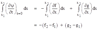
If we choose, instead, to deal only with the combined wave function, we must still specify a second function to enable us to infer the values at arbitrary events. To play the role of this second function, it is traditional to specify the time-derivative of the combined wave function. Thus we are typically “given” the values of ψ and ∂ψ/∂t along the entire x axis. It is somewhat more difficult to infer from these two functions, rather than from the components f and g, the value of the wave function at an arbitrary event. Essentially we need to isolate the two components so that we can project them to the desired event. The values of the wave function on the “past light cone” are not sufficient to do this – even though the components on the past light cone are sufficient. By encoding our “given” information in terms of the combined wave function and its time derivative on the x axis, we have made it necessary to infer the decomposition of the wave function by integrating the derivative values from one projection line to the other. We have

Integrating this along the line t = 0 (i.e., the x axis) between the two points x₁ and x₂ that are light-like projections from the event in question onto the x axis, we get

where subscripts signify the locations, x₁ or x₂, on the x axis. Of course, we also have

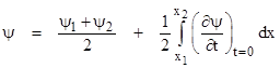
so we can add this difference to the previous integral to give 2(g₂ – g₁). Consequently, taking half of this, and adding it to ψ₁ = f₁ + g₁ gives (finally!) the desired result, which is just f₁ + g₂.  Thus we have the traditional “solution” of the one-dimensional wave equation

On this basis it is sometimes said that Huygens’ Principle does not apply in one space dimension, because this equation suggests that the wave function at an arbitrary event depends on the values inside its past light cone, represented by the range of the integral in the above expression. However, as we’ve seen, it is only because we chose to encode our boundary conditions in terms of two particular functions that we were led to this expression. If, instead, we express our conditions in terms of the two component functions, we find that the wave function at an arbitrary event is indeed determined fully by the conditions on the past light cone.

This should serve as a cautionary example of how misleading it can be to infer causal structure from the form of an expression for the wave function. Any such expression actually represents only a set of correlations, not necessarily indicative of an underlying causal flow. This can be even more vividly illustrated by noting that the expressions derived above are applicable not just to events at later times, but also to past events. In other words, we can use those same expressions, based on the boundary conditions specified at t = 0, to compute the wave function for an event at any time prior to t = 0, in terms of the values of the wave function on the future “light cone” of that event. Do we infer from this that the future conditions are the cause of the past conditions? Ordinarily we do not, we simply recognize the existence of correlations between the wave function (and its derivatives) at certain sets of points, and it is possible to infer the values of the wave function at some points gives the values at some other points.

Another, equally valid, way of imposing boundary conditions is to specify the functions along the t axis at x = 0. Again the most efficient method is to specify the positive and negative-going components f and g for every point along this axis, enabling us to determine the combined wave function for any arbitrary event. However, on this basis, the wave function at each event is seen as being determined by the “retarded” component f specified for a point at the spatial origin in the past, and the “advanced” component g specified for a point at the spatial origin in the future. Again, we need not (an usually do not) interpret this to mean that information or physical effects are flowing backwards in time. This is merely another of the infinitely many sets of correlations that exist between the values of the wave function at various times and places.

To this point we’ve focused on the wave equation in just a single space dimension, and found several different formulations, each of which might superficially be thought to imply very different causal structures. When we proceed to higher dimensions, we introduce a new feature, related to the question of whether waves are to be regarded as ultimately attributable to a singular particle, or whether we need to allow for the possible existence of coherent waves that don’t arise from a single point-like source. With just a single space dimension, the only distinction between a plane wave and a “spherical” wave is that a plane wave consists of a single wave moving in just one direction, whereas a “spherical” wave consists of two symmetrical waves emanating outward from the origin. In our discussion of the one-dimensional case we referred to individual waves propagating in both directions, so we didn’t actually consider “spherical” waves. In higher dimensions we can represent spherical waves by restricting ourselves to spherically symmetrical solutions of the wave equations. The spatial coordinates are then represented by a single non-negative radial coordinate r, signifying the spatial distance from the unique center of the wave. As shown in the article on Huygens’ Principle, the general spherically symmetrical solution of the wave equation in three space dimensions is

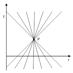
where, just as in the one-dimensional case, the functions F and G are arbitrary. However, unlike the x coordinate in one-dimensional space, the r coordinate in three dimensional space is not symmetrical in the increasing and decreasing directions. This is obvious from the fact that we regard negative r values as unphysical. Also, a wave propagating in the positive r direction is expanding outward and becoming less intense (because of the r in the denominator), whereas a wave propagating in the negative r direction is contracting inward and becoming more intense. The pattern of correlations along “light-lines” is essentially the same as in the one-dimensional case, except the bi-directional x coordinate is replaced with the uni-directional r coordinate, as shown below.

We now have the familiar choices as to how to express the solutions, i.e., how to give the value of the wave function at an arbitrary event in terms of the value at certain other events. However, in this context, some of the alternatives seems distinctly implausible from a physical point of view. We could, for example, impose the required boundary conditions by specifying the inward and outward wave components for every radius r at the initial reference time t = 0. (We could normalize these by multiplying each value by the radius r.) The wave function at the point P would then be the sum of F(1) and G(5), divided by r = 3. We aren’t nearly as tempted in this situation to take the condition at B as the physical origin of the inward wave, because B is not a point, it is a spherical surface, and it’s hard to imagine any physical circumstance that would produce a spherically symmetrical inward-propagating wave. In fact, we could make similar comments about the spherical surface A as the physical original of the outward-going wave. In the outward case we would almost certainly trace the actual physical cause of F(1) further into the past, to the point denoted by C at the center. Likewise we could assign the physical origin of G(5) to the point denoted by D at the center. However, this implies that the G components are advanced waves, propagating from the future into the past, contrary to our usual expectation.

The conventional attitude in this situation is to discount the physicality of advanced waves propagating from the future into the past, and to explain the (usual) absence of inward-propagating spherical waves simply by noting that the conditions to produce such a wave are extremely rare, even though (in principle) such waves could exist. So, for a spherically symmetrical situation, we conventionally assume that the G components are all zero, and the field consists entirely of the “retarded” F component, which we regard as emanating outward, and into the future, from the center of the field. (There have, of course, been occasional proposals to incorporate advanced waves into physical theory, such as the Wheeler-Feynman theory of electrodynamics, but these haven’t become part of standard physical explanations.)

More generally we allow for multiple sources of waves at various locations, and all these fields can be superimposed without interfering with each other. So, in order to fully define the wave function at a given point, we need to consider the retarded waves emanating from every direction on its past light cone. This is consistent with the Lenard-Weickart potential of electromagnetism, which is determined by the charges residing on the past light cone.

So far we’ve considered wave propagation in one and in three spatial dimensions, but not in two dimensional space. As explained in the note on Huygens’ Principle, the propagation of waves in a space with an even number of dimensions differs in a profound way from wave propagation in space with an odd number of dimensions, because with an even number of space dimensions the solution cannot be expressed purely in terms of scaled functions of  r – t  and  r + t. Thus the strong form of Huygens’ Principle is not satisfied. With regard to causation, though, it’s interesting to examine closely the different ways in which the solutions in two space dimensions can be expressed.

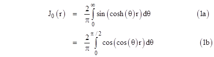
We typically separate the time and space variables, and find that the time portion is a simple harmonic equation satisfied by sin(t), whereas the solution of the spatial portion is the Bessel function J₀(r), so the total wave function has the form sin(t)J₀(r). (This is for standing waves that are free of singularity at the origin; for solutions with singularities at the origin, the Bessel function J₀ is replaced with the Hankel function H₀, also known as a Bessel function of the third kind.) Now, the Bessel function has the following two useful integral representations

Equation (1b) is valid for any complex r, and equation (1a) is valid for all real r greater than zero, so each of these expressions covers the domain of interest. However, as indicators of the causal structure of the wave function, these two expressions are profoundly different. Expression (1a) is very much what we would expect, familiar as we are with the traditional view of the causal structure of spacetime, because when we multiply through by sin(t) and making use of trigonometric identities we get a complete wave function of the form

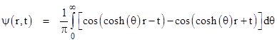
Thus instead of being a function of the quantities r ± t (as in the odd-dimensional cases), we find that the solution is a function of  cosh(θ)r ± t, where θ varies from 0 to infinity, so the characteristic “propagation speeds” are not just  ±1, but are  ±1/cosh(θ), which means the relevant speeds range from unity down to zero. We can interpret this as signifying that the wave function as a given event depends not just on the wave function on the past “light cone” of that event, but on the interior of the past light cone. Indeed this is the standard conclusion for even-dimensional spaces, i.e., they do not exhibit “sharp” wave propagation. Of course, we typically choose just the retarded component, in order to say the wave propagates from the past into the future. The putative causal “flow” for the event at P is depicted in the figure below.

However, expression (1b) is just as valid a representation of the Bessel function (and is a finite integral with a larger domain of convergence), and if we again multiply through by sin(t) we get the following equally valid expression for the total wave function

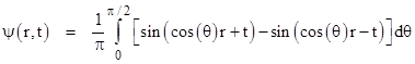
This is perfectly identical to the previous wave function, but it is explicitly a function of the quantities  cos(θ)r ± t, where θ varies from 0 to π/2, so the characteristic propagation speeds are  ±1/cos(θ), which means the relevant speeds range from unity to infinity. This implies that the wave function at any given event is determined by the rays impinging on that event from the exterior of the “lightcone”, which might be taken to suggest that the causal structure is precisely the complement of the causal structure that we inferred from the previous expression. This alternate structure of dependency for an event at P is depicted below.

These examples show how misleading it can be to assume that a set of events (or rays) that determine the wave function at a given event are the source or cause of the wave function at that event. Our choice of the interior rays of the light cone (rather than the exterior) as the correct “causal” interpretation is justified and motivated largely by the existence of identifiable particles on time-like trajectories, which guarantees the each successive causal past (for a given particle) is a superset of all the previous causal pasts. This would obviously not be true if we chose the exterior rays – unless we took the radical step of identifying space-like separated instances of (say) electrons as an individual entity. In normal circumstances this would not be a very viable alternative, because the overlap between the wave functions of separate particles is typically very small, but in extreme conditions it’s conceivable that the most viable identifications of worldlines might change from timelike to spacelike. For example, something very much like this occurs at the Schwarzschild radius of a particle of matter in the classical field theory of general relativity, where the spacelike and timelike directions are exchanged. In that circumstance, we again find that the “causal past” of each successive instance of a particle is a superset of all the prior causal pasts, but now this comprises a toroidal region converging on the central point. It’s interesting to consider how, in the context of overlapping wave functions of identical particles, the most viable “topology of contiguity” could change in some regions of extremely high density, such as in a strong gravitational field. This is indicated pictorially in the figure below.

The left-most figure shows many instances of an identical particle such as an electron. Each dot signifies the center of a wave function. The central figure shows how we would most likely identify the worldlines of “individual particles”, and how, at some region of high spatial and low temporal density, the most plausible identifications could switch from timelike to spacelike. The right-most image is intended to convey the varying degrees of overlap between the wave functions of the discrete instances of the particle, showing what we would regard as two separate individuals in the lower graph, and a single propagating individual in the upper graph.

Another interesting aspect of the wave equation is its formal similarity to the Laplace equation, whose solutions are harmonic functions. How would we describe the “causal structure” of these solutions? Recall that the Laplace equation in three dimensions is

As discussed in the note on the Divergence Theorem, the solutions of this equation are such that the value of ψ(x,y,z) at any given point equals the average of ψ(x,y,z) over any sphere centered on that point. In other words, we have

where the integral is evaluated over the surface of the sphere of radius R centered on the point x,y,z. More generally, the function inside any given region is completely determined by the function on the boundary of that region. Clearly we can’t identify a unique causal flow for a solution of the Laplace equation, because every point is, in a sense, symmetrical with every other point, just as every direction in the space is symmetrical with every other direction. The equation establishes correlations and relationships between separate points, but doesn’t (by itself) imply a unique causal structure. In contrast, the wave equation in one space dimension is

Despite the formal similarity to the Laplace equation, the solutions of this equation have a significantly different character. Nevertheless, it’s natural to ask if the solutions of this equation satisfy a relation analogous to (2). Indeed they do, as can be seen by superimposing arbitrarily many spherically symmetrical solutions. Suppose every point X,Y,Z in a three dimensional space is quiescent prior to t = 0, and at time t = 0 is the origin of a retarded spherical wave pulse (a supposition that accords with Huygens’s Principle) of the form

where F is an arbitrary function, δ is the “delta function”, and r_XYZ is the distance from x,y,z to the center of the wave X,Y,Z, so we have

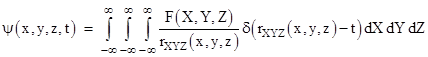
The total wave function at x,y,z is the superposition of all these contributions, given by the integral

The defining property of the delta function is

so the only non-zero contributions in the triple integral occur with r_XYZ = t, and hence we need only integrate over the X,Y,Z values such that r_XYZ = t for the given x,y,z. This locus is a spherical surface of radius t centered on the point x,y,z, which means it consists of the points

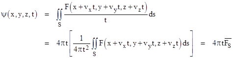
Thus the triple integral can be replaced by the double integral over this surface

where  denotes the mean value of F on the sphere S. In other words, ψ(x,y,z,t) is a solution of the wave equation if it equals  4πt  times the average value of F over the spherical surface of radius t centered on the spatial point x,y,z. If F is bounded, it follows immediately that ψ(x,y,z,0) = 0. Also, if F is a smooth function, the average value of F on spheres centered on a given point is independent to the first order of the radius around a radius of zero, and of course that average equals (to the first order) the value of F at the central point, so we have

Thus, given boundary conditions of the form ψ(x,y,z,0) = 0 and some function

we have a solution

where ϕ(x,y,z) may be specified freely. We also know that, since partial differentiation is commutative, any partial derivative of a solution of the wave equation is also a solution. For example, letting subscripts denote partial differentiation, if y is a solution of the wave equation

then ψ_t is also a solution, because

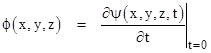
Therefore, another solution of our original wave equation is given by the partial derivative of the previous solution with respect to time, i.e.,

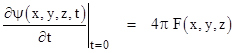
where φ(x,y,z) may be freely specified. Again if φ is a smooth function, the average value on the sphere S is constant to first order at t = 0, so we have

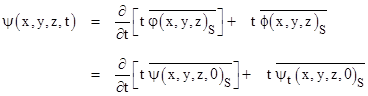
Combining these two solutions gives a complete solution to the Cauchy initial value problem, i.e., given the values of ψ and ψ_t for the entire initial timeslice t = 0, the resulting wave function is

This confirms that the wave function at a given event is fully determined by the conditions on the past light cone of the event, which is the sphere S at time t = 0. Of course, this derivation was based on the stipulation that only the retarded part of the general spherical solution would be considered. Also, as we saw previously, the wave function is also fully determined by the conditions in certain other regions (the Cauchy initial value formulation is to some extent arbitrary), so again we cannot assert a unique flow of cause and effect. This ambiguity is unavoidable in any fully deterministic context.

Return to MathPages Main Menu