The Euler-Maclaurin Formula

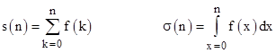
One of the fundamental concepts of calculus is the correspondence between sums and integrals. Given any sufficiently well-behaved continuous function f(x), consider the sum the integral defined by

These two functions obviously have some similarities, but they also have significant differences. For example, the summation is taken over the values of f(k) at discrete integer arguments k = 0, 1, 2, …, n, whereas the integral is taken over the values of f(x) for arguments x varying continuously from 0 to n. Strictly speaking, the function s(n) is defined only for integer arguments, while σ(n) is defined for any non-negative real value of n. Nevertheless, we can derive an interesting and useful relation between these two functions.

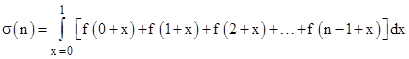
First, notice that σ(n) can be written in the form

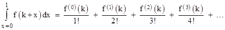
The Taylor series expansion of each of the individual terms of the integrand is of the form

where f^(j) denotes the jth derivative of f. The integral of this term from x = 0 to 1 is

Inserting all these expressions into the original integral, we get

where

Now, if we had started with the derivative of f in place of f, we would have arrived at the same expression (1), except that each f ^(j) would be replaced with f ^(j+1), and hence each S^(j) would be replaced with S^(j+1), and σ(n) would be replaced with σ⁽¹⁾(n) where

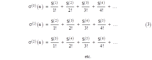
Thus beginning with successively higher derivatives of f, we get the infinite sequence of relations

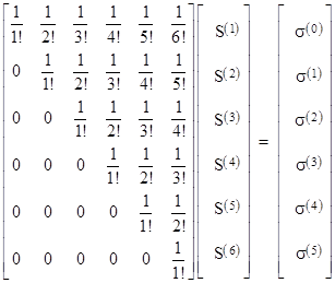
Each of these equations has (in general) infinitely many terms, but we can solve the system of equations for any finite numbers of terms by taking just a restricted portion of these equations. For example, taking just the terms up to S⁽⁴⁾ from the first four equations, we have (in matrix form)

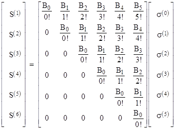
Solving this system of equations gives

where

and so on are the Bernoulli numbers. Thus we have

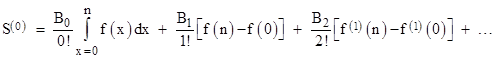
Inserting the expressions for each σ^(j) from equation (2), this gives

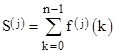
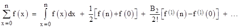
Recall that S⁽⁰⁾ is defined as the sum of f(k) for k = 0, 1, 2, …, n-1. Therefore, if we wish to express this in terms of a summation from k = 0 to n, we must add f(n) to both sides. Noting that B₁ = -1/2, this leads to the result

This is called the Euler-Maclaurin formula, a generalization of Bernoulli’s formula for the sum of powers of the first n integers. We should note that this series is divergent for most applications, but the error is less than the first neglected term, so the Euler-Maclaurin formula is often a useful method of approximation, relating the series summation to the continuous integral of a function.

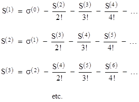
Incidentally, by examining the inversion of the system of equations (3) in detail, we can gain some insight into the structure of the Bernoulli numbers, as well as the more general Bernoulli polynomials. First, we re-write equations (3) in the form

where we have omitted the argument “(n)” from the σ^(k) terms for convenience. These equations show the beginnings of how to express each S^(j) as a function of the σ^(k)(n) terms, and we must now repeatedly substitute from the left-hand side into the right side to eliminate higher and higher derivatives of S from the equation for S⁽¹⁾. Our objective now is to determine the coefficients of the σ^(j) terms in the expression for S⁽¹⁾ once all the higher S derivatives have been eliminated. Clearly the coefficient of σ⁽⁰⁾ will be 1, because none of the remaining terms contain any occurrences of that quantity. Also, we can see that the coefficient of σ⁽¹⁾ will be -1/2, which arises from substituting the expression for S⁽²⁾ into the first equation. No other substitutions will give any more occurrences of that quantity.

In general, the coefficient of σ^(j) will be the sum of products of the reciprocal factorials involved in the sequence of substitutions leading to the occurrence of that term in the first equation. For example, the term σ⁽²⁾ reaches the first equation in two ways. First, it appears directly when we substitute S⁽³⁾ into the first equation, and this appearance has a coefficient of -1/3!. Second, it appears when we substitute S⁽³⁾ into the second equation, where it is given a coefficient of -1/2!, and then this S⁽²⁾ is substituted into the first equation, where it is given another factor of -1/2!. Consequently, the overall coefficient of σ⁽²⁾ in the final expression for S⁽¹⁾ will be -1/3! + (1/2!)² = 1/12. Likewise the coefficient of σ^(k) for any k consists of the sum of 2^k-1 products of negative reciprocal factorials, corresponding to the distinct partitions of k (including order).

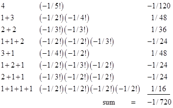
For example, the coefficient of σ⁽⁴⁾ is given by the sum of the eight products shown below along with the corresponding partitions of 4:

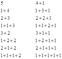
The sum in this case is, of course, simply B₄/4!. The fact that there are 2^k-1 of these partitions follows because there are k-1 possible locations for slicing the interval from 0 to k, and each of these slices can either be present or absent. We can now express the nth Bernoulli number as an explicit sum of products of (signed) reciprocal factorials, although the number of summands doubles for each successive Bernoulli number, so this formula isn’t of much practical value. However, notice that the partitions on each level can be generated very simply from those on the previous level. We can generate the first half of the partitions on the next level by simply incrementing the last components of each partition on the current level. Then we can general the other half of the partitions on the next level by simply appending a “1” to each partition on the current level. Thus the sixteen partitions involved in determining the coefficient of σ⁽⁵⁾ are as shown below.

It’s also easy to adjust the product corresponding to each of these partitions, and the same adjustment factor applies to each partition ending in the same number. So, it will be convenient to represent each Bernoulli number B_k as the sum

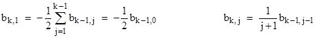
where b_k,j denotes the sum of the products in the expression for B_k whose corresponding partitions end with j. If we let b_k,0 denote B_k, then we have the simple relations

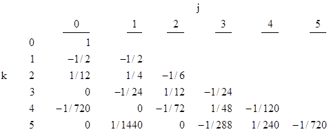
Using these relations we can generate the table below.

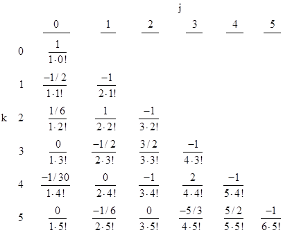
The values in this table can also be presented with suitably chosen scale factors as shown below, revealing that not only are the b_k,0 terms (which are the sums of all the other terms in the respective rows), but the b_k,j terms are scaled version of the coefficients of the Bernoulli polynomials.

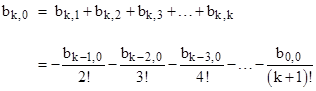
Since each number in the j = 0 column is the sum of the other elements in that row, and since those other elements can be expressed by reciprocal factorials, it follows that there is a recursive relation involving just the elements in the j = 0 column (i.e., the standard Bernoulli numbers).  From the previous recurrence relations we have

Therefore we have

Since the terms in the j = 0 column are the standard Bernoulli numbers scaled according to B_k/k! = b_k,0, this represents the equation

Multiplying through by (k+1)!, we get the familiar form of the recurrence

Return to MathPages Main Menu