Eigen Duality and Quantum Measurement

For a given square matrix M an eigenvector is a vector x such that the multiplication of x by M simply re-scales x while leaving the direction of x unchanged. In other words, x is an eigenvector of M if and only if Mx = λx for some scalar λ, which is called the eigenvalue corresponding to x. This condition can also be written in the equivalent form

where I is the identity matrix and 0 is the zero vector. Naturally the equation is trivially satisfied by x = 0, but the equation may also have non-trivial solutions if the determinant of the operator is zero. This requires that λ be a root of the characteristic equation

which is a polynomial in λ of degree equal to the order of the matrix M. If we multiply through equation (1) by (−y₂/λ)M₂ for some arbitrary scalar y₂ and square matrix M₂ we get the equivalent expression

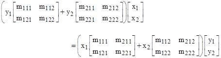
where y₁ = −y₂/λ and M₁ = M₂M, but now the “eigenvalue” is represented by two numbers, y₁ and y₂, instead of just the single number λ. Of course, only the ratio of these two numbers is significant, so each eigenvalue λ is represented by a ray through the origin of the y₁,y₂ plane. Although equation (3) is equivalent to (2), it highlights an important and profound symmetry, because it shows that there is no difference between eigenvalues and eigenvectors. To make this explicit, consider the simple case where M₁ and M₂ are square matrices of order 2, and x is a column vector with two components x₁ and x₂. Letting m_1ij and m_2ij denote the elements of M₁ and M₂ respectively, we can multiply out the left side of equation (3) explicitly and show that it can be written in either of two forms:

When written in the first form, y₁ and y₂ are the numerator and denominator of the eigenvalue, and x₁ and x₂ are the components of the eigenvector. But when written in the second form, the roles are reversed, i.e., y₁ and y₂ are the components of the eigenvector, and x₁ and x₂ are the numerator and denominator of the eigenvalue. (Note that only the direction of an eigenvector is constrained by the system of equations, so only the ratio of its components is significant, just as only the ratio of the numerator and denominator of the eigenvalue is significant.) Of course, the coefficient matrices are decomposed differently, in one case being of the form m_1ij and m_2ij, and in the other case being of the form m_ji1 and m_ji2 respectively, but this simply reflects the fact that x and y lie in different component spaces. There is no justification for giving either of them priority over the other.

The duality between eigenvalues and eigenvectors applies for systems of any order. It is simply disguised in most applications because we artificially break the symmetry by forcing one of the matrices to be the identity and forcing the scalar multiplier of the other matrix to be unity. This not only obscures the natural duality between eigenvectors and eigenvalues, it also entails an unwarranted specialization of the general form by not allowing additive partitions of the coefficient matrix. In addition, writing the equation in the symmetrical form suggests two interesting mathematical generalizations, and also has some interesting relevance to the interpretation of physical theories, especially quantum mechanics. We discuss each of these topics below.

First, to clarify the symmetry between eigenvalues and eigenvectors, we will define a notation and index convention for matrices and vectors. We’re accustomed to dealing with two different kinds of vectors, which we may call column and row vectors, but these are just two of infinitely many possible kinds of vectors, one for each of the possible dimensions of an array. Let us combine the two original matrices M₁ and M₂ into a single three-dimensional matrix, denoted by M_μνσ where μ,ν,σ are indices ranging from 1 to 2, and let X_μ11 denote the vector with elements x₁₁₁ = x₁ and x₂₁₁ = x₂ (the components of the eigenvector x), and let Y_1ν1 denote the vector with elements y₁₁₁ = y₁ and y₁₂₁ = y₂. In general we indicate multiplications using the summation convention over repeated indices in a single term. Also, if corresponding indices of two arguments are both explicit numerals, or both dummy indices, we set that index of the product to 1, whereas if the index is a numeral or dummy (repeated) in one argument but a variable in the other, we set that index of the argument to the variable. To illustrate, the product P given by ordinary matrix multiplication of the original two matrices could be expressed as

With this notation, our eigenvalue system is written in the form

Since X and Y are orthogonal, they commute. Thus this eigenvalue problem, when expressed in its natural symmetrical form, simply consists of finding two vectors that, when used as relative weights for summing and contracting a three-dimensional array in two of its dimensions, yields a zero vector in the remaining dimension. Of course, we could also multiply by a vector in the third dimension to collapse the matrix down to a scalar 0, which would result in a continuous locus of eigen-solutions. For any choice of one of those three vectors, the remaining two would have two discrete solutions (up to the arbitrary scale factors).

It might seem as if the duality between eigenvalues and eigenvectors exists only for matrices of order 2, because there are only two terms in the traditional eigenvalue equation (3), with coefficients representing the numerator and denominator of the traditional scalar eigenvalue. However, the symmetrical form immediately leads to a natural generalization of (3), such that we can partition the operator into more than just two parts. For example, by partitioning the coefficient matrix into three parts (instead of just two), we have a system described by the equation

where A, B, C are square matrices of order N, and α, β, γ are scalars. As before, this equation can have non-trivial solutions only if the determinant of the overall operator vanishes, i.e.,

This represents a polynomial of degree N in the three scalars α,β,γ. Again, only the ratios of these components are significant, so the “eigenvalues” of the system consist of rays through the origin of a three-dimensional space, just as (if N = 3) the eigenvectors are rays through the origin of a three-dimensional space. If we normalize the projective space of the eigenvalues (which we can do in various ways, such as by dividing through the characteristic equation by the Nth power of one of the eigen-components, or by stipulating that α + β + γ = 1), we get a quadratic equation in two variables, so the eigenvalues now consist of a conic locus of points on the normalized surface. An alternative is to normalize the length of the eigenvalue to unity, i.e., to stipulate that α² + β² + γ² = 1, in which case the eigenvalues consist of a continuous locus of points on the unit sphere in three dimensions – as do the normalized eigenvectors.

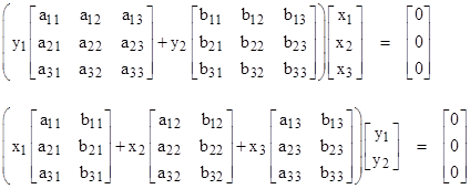
By partitioning the coefficient matrix into N parts, we get a system with N-dimensional eigenvalues and N-dimensional eigenvectors, and the coefficient matrices are N x N square matrices regardless of whether we transpose the eigenvalues and eigenvectors. However, the duality between eigenvalues and eigenvectors is not limited to such cases. In general we can have different numbers of dimensions for those entities. For example, consider a system described by

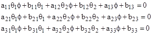
where the two coefficient matrices A and B are of order three. In this case the system equations can be written explicitly in either of the following two equivalent forms

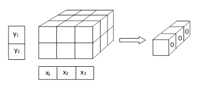
Thus the duality between x and y still applies, in the sense that either of those “eigenrays” can equally well be regarded as the eigenvalue or the eigenvector, with the understanding that the coefficient matrices need not be square. The operation represented by these expressions can be depicted schematically as shown below.

This shows that, beginning with a 2 x 3 x 3 coefficient array, we collapse this matrix in the vertical dimension by applying the y vector components as weight factors, summing the elements in each vertical column, leaving a 3 x 3 array, which we then collapse in the second dimension by applying the x vector components as weight factors, summing the elements of each row. The result is a one-dimensional vector, which we require to be null.

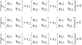
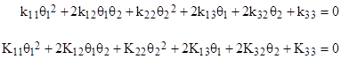
Of course, if the coefficient matrices are not square, the eigen condition can no longer be expressed as the vanishing of the determinant of the sum of the coefficient matrices, because the definition of the determinant applies only to square matrices. Nevertheless, we still have a perfectly well-defined eigen condition, with the understanding that it consists, in general, of a set of simultaneous equations rather than just a single equation. In the above example, the eigen condition on y is expressed by the vanishing of the determinant of the sum of the two square coefficient matrices, which implies just a single polynomial in the y_j parameters, whereas the eigen condition on x consists of any two of the three simultaneous conditions

In this example the basic system equations (6) represent three expressions being set to zero (the three components of the right hand side), and there are five unknowns, but since the equations are homogeneous we can divide through by y₂ and x₃, leading to the following three equations in the three unknowns θ₁ = x₁/x₃, θ₂ = x₂/x₃, and ϕ = y₁/y₂.

Solving the first equation for ϕ gives

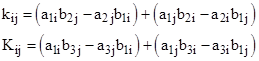
Substituting this into the other two equations, we get two conic equations

where

The solutions consist of the four points of intersection (θ₁,θ₂) between these two conics, and for each of these four (possibly complex) solutions the corresponding value of ϕ is given by the previous equation. One might think that this is inconsistent with the fact that equation (6) has just three distinct eigen solutions, rather than four. The explanation is that one of the four “eigenvalues” ϕ is infinite. To see this, note that ϕ is infinite when the denominator in the expression given above equals zero, which is to say

Solving this for θ₂ and substituting into the two conic equations, we find that they both factor as products of two linear expressions, and the two conics share a common factor, so we always have the “fourth solution”

This shows that the usual formulation is not fully general, because it excludes this “fourth solution”, whereas the variable ϕ is actually the ratio x₁/x₂, so this fourth solution simply represents the case x₂ = 0. Incidentally, the remaining linear factors of the two conics are equal to each other if and only if the determinant of the “a” matrix vanishes.

To illustrate the duality between X and Y even more clearly, consider the system of equations

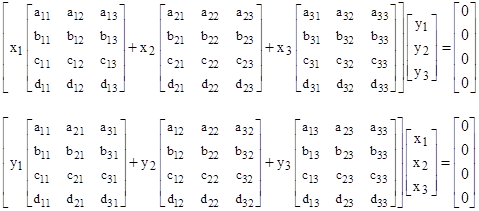
In this case, using the symbols a_μν = M_μν1, b_μν = M_μν2, and so on, we can write the system equations explicitly in either of the two equivalent forms

Assuming x₃ and y₃ are not zero, we can divide through these homogeneous equations by x₃y₃, leading to four equations in the four unknown ϕ₁ = x₁/x₃, ϕ₂ = x₂/x₃, θ₁ = y₁/y₃, and θ₂ = y₂/y₃. We can solve the first two equations for θ₁ and θ₂ as ratios of quadratic expressions in ϕ₁ and ϕ₂. Likewise we can solve the last two equations for θ₁ and θ₂, and we can then equate the corresponding expressions to give two quartics in ϕ₁ and ϕ₂. The overall solutions are then given by the intersections of these two quartics. As discussed in the note on Bezout’ theorem, there are 16 points of intersection between two quartics, counting complex points, multiplicities, and points at infinity.

As a further generalization, we need not be limited to systems with just two “eigenrays” (i.e., systems with eigenvalues and eigenvectors). Using the index notation discussed previously, we can define overall coefficient matrices with any number of dimensions, and then contract it with two or more eigenrays. For example, we can consider systems such as

where the indices α,β,γ,δ need not all vary over the same ranges. Each of the vectors X, Y and Z represents a class of eigenrays for the system. The vectors X,Y,Z can be regarded as weight factors that are used to collapse the M array down to a lower number of dimensions. Even more generally, we can consider “eigenplanes”, etc., by allowing the X “vectors” to be of more than just one dimension. For example, we can consider systems such as

These examples show that the artificial distinction between eigenvalues and eigenvectors is completely meaningless. A good illustration of this is given by the simplest expression of this form, namely

where the indices range from 1 to 2. This represents the single constraint

In terms of the ratios ϕ = x₁/x₂ and θ = y₁/y₂, this can be written as

Thus we can regard the ratio (x₁/x₂) as the eigenvalue corresponding to the eigenvector [y₁,y₂], and conversely we can regard the ratio (y₁/y₂) as the eigenvalue corresponding to the eigenvector [x₁,x₂], and these ratios are related by a linear fractional (Mobius) transformation. Of course, this simple system doesn’t restrict the set of possible eigenvalues or eigenvectors, but it does establish a one-to-one holomorphic mapping between them. Even this simple system has applications in both relativity and quantum mechanics, since the Mobius transformations can encode Lorentz transformations and rotations, and with stereographic projection onto the Riemann sphere they can be used to represent the state vectors of a simple physical system with two basis states.

Equation (7) represents a two-dimensional coefficient matrix being collapsed in both dimensions down to a single null scalar, but we can also begin with a three-dimensional coefficient matrix and collapse it in two dimensions down to a one-dimensional null vector. This is represented by the equation

Again letting x_α denote X_α11 and so on, this corresponds to the two conditions

and in terms of the ratios ϕ = x₁/x₂ and θ = y₁/y₂ these can be written as

Equating these two values of ϕ, we get a quadratic condition for θ, defining the two eigenvalues, but these can equivalently be regarded as the ratios of the components of the two eigenvectors, and the same applies to the corresponding values of ϕ.

One could argue that the conventional expression of problems in terms of eigenvalues and corresponding eigenvectors is due to the constraint on the degrees of freedom that this arrangement imposes on the results. Suppose we have a rectangular array of size a x b x c, and we collapse the array in the a and b directions, leaving just a vector of size c. This represents c homogeneous constraints, and we can divide through these equations to give a-1 and b-1 variables. To make this deterministic (up to the multiple roots), we must have a + b – 2 = c. Thus if either a or b is equal to c (to make square matrices of the bc planes), then the other must equal 2, suggesting that it be treated as an eigenvalue. However, we need not restrict ourselves to cases when all the continuous degrees of freedom are constrained. In fact, there are many real-world applications in which there are unconstrained continuous degrees of freedom. Also, as noted above, we need not restrict ourselves to square matrices.

So far we’ve considered only purely mathematical generalizations of eigenvalue problems, but another kind of generalization is suggested by ideas from physics. The traditional asymmetrical form Mx = λx used in the representation of a “measurement” performed by one system on another in the context of quantum mechanics gives priority to one of the two interacting systems, treating one as the observer and the other as the observed. But surely both systems are “making an observation” of each other (i.e., interacting with each other), so just as there is an operator M₁ representing the observation performed by one system, there must be a complementary operator M₂ representing the reciprocal “observation” performed by the other system. This strongly suggests that the symmetrical form, with some non-trivial partition of the coefficient matrix, is more likely than the asymmetrical form to give a suitable representation of physical phenomena. According to this view, the eigenvalue arising from the application of an observable operator is properly seen as part of the state vector of the “observing system”, just as the corresponding state vector to which the “observed system” is projected can be seen as the “value” arising from the measurement which the “observed system” has performed on the “observing system”.

To fully establish the equivalence between eigenvalues and eigenvectors in the context of quantum mechanics we need to reconcile the seemingly incongruous interpretations. The eigenvector is associated with an observable state of a system, and its components are generally complex. To give these components absolute significance (as probability amplitudes) they are normalized by dividing each component by the square root of the sum of the squared norms of all the components (so that the sum of the squared norms of the normalized components is unity). In contrast, the eigenvalue – regarded as the purely real scalar result of a measurement – is the ratio of the two components of the representative eigenvector. In other words, given the vector components z₁ and z₂, we traditionally take the ratio λ = z₁/z₂ as the physically meaningful quantity, i.e., the result of a measurement, whereas if we regarded this vector as an eigenvector we would take the quantity z₁/(|z₁|² + |z₂|²)^1/2 and its complement as the physically meaningful quantities, namely, the probability amplitudes for states 1 and 2. This seems to suggest the following mapping between the eigenvalue λ the state probabilities P₁, P₂ for a given vector:

and hence the ratio of probabilities is P₂/P₁ = λ².

For more on this subject, see Eigen Systems. Also, another generalization of eigen-value problems is discussed in the note on quasi-eigen systems.

Return to MathPages Main Menu