Analytic Continuation

If as many numbers as we please be in continued proportion, and there be subtracted from the second and the last numbers equal to the first, then, as the excess of the second is to the first, so will the excess of the last be to all those before it.

                                                          Euclid’s Elements, Proposition 35, Book 9

As Euclid discussed in the Elements, a series of geometrically increasing numbers

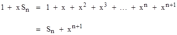
can be expressed in terms of just the second and the last number by noting that

Solving for S_n gives

Now, if the magnitude of x is less than 1, the quantity xⁿ⁺¹ goes to zero as n increases, so we immediately have the sum of the infinite geometric series

Archimedes evaluated the area enclosed by a parabola and a straight line essentially by determining the sum of such a series. This is perhaps the first example of a function being associated with the sum of an infinite number of terms. To illustrate, if we set x equal to 1/2, this equation gives

There is, of course, a very significant difference between equations (1) and (2), because the former is valid for any value of x, whereas the latter clearly is not… at least not in the usual sense of finite arithmetical quantities. For example, if we set x equal to 2 in equation (2) we get

which is surely not a valid arithmetic equality in the usual sense, because the right side doesn’t converge on any finite value (let alone -1). This shows that the correspondence between a function and an infinite series such as (2) may hold good only over a limited range of the variable. Generally speaking, an analytic function f(z) can be expanded into a power series about any complex value of the variable z by means of Taylor’s expansion, which can be written as

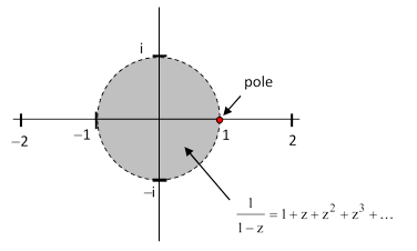
but the series will converge on the function only over a circular region of the complex plane centered on the point z₀ and extending to the nearest pole of the function (i.e., a point where the function goes to infinity). For example, the function f(z) = 1/(1-z) discussed previously has a pole at z = 1, so the disk of convergence of the power series for this function about the origin (z = 0) has a radius of 1. Hence the series given by (2) converges unconditionally only for values of x with magnitude less than 1. This is depicted in the figure below.

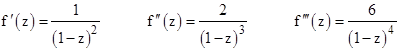
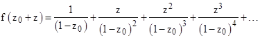
The analytic function f(z) = 1/(1-z) can also be expanded into a power series about any other point (where the function and its derivatives are well behaved). The derivatives of f(z) are

and so on. Inserting these into the expression for Taylor’s series we get

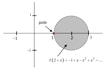
Hence the power series for this function about the point z₀ = 2 is

Each of the power series obtained in this way is convergent only on the circular region of the complex plane centered on z₀ and extending to the nearest pole of the function. For example, since the function f(z) = 1/(1-z) has a pole at z = 1, the power series with z₀ = 2 is convergent only in the shaded region shown in the figure below.

So far we’ve discussed only the particular function f(z) = 1/(1-z) and we’ve simply shown how this known analytic function is equal to certain power series in certain regions of the complex plane. However, in some circumstances we may be given a power series having no explicit closed-form expression for the analytic function it represents (in its region of convergence). In such cases we can often still determine the values of the “underlying” analytic function for arguments outside the region of convergence of the given power series by a technique called analytic continuation.

To illustrate with a simple example, suppose we are given the power series

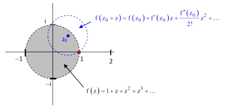
and suppose we don’t know the closed-form expression for the analytic function represented by this series. As noted above, the series converges for values of z with magnitudes less than 1, but it diverges for values of z with magnitudes greater than 1. Nevertheless, by the process of analytic continuation we can determine the value of this function at any complex value of z (provided the function itself is well-behaved at that point). To do this, consider again the region of convergence for the given power series as shown below.

Since the known power series equals the function within its radius of convergence, we can evaluate f(z) and its derivatives at any point in that region. Therefore, we can choose a point such as z₀ shown in blue in the figure above, and determine the power series expression for f(z₀ + z), which will be convergent within a circular region centered on z₀ and extending to the nearest pole. Thus we can now evaluate the function at values that lie outside the region of convergence of the original power series.

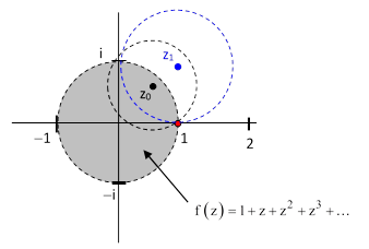
Once we have determine the power series for f(z₀ + z) we can repeat the process by selecting a point z₁ inside the region of convergence and determining the power series for f(z₁ + z), which will be convergent in a circular region centered on z₁ and extending to the nearest pole (which is at z = 1 in this example). This is illustrated in the figure below.

Continuing in this way, we can analytically extend the function throughout the entire complex plane, except where the function is singular, i.e., at the poles of the function.

In general, given a power series of the form

where the a_j are complex coefficients and α is a complex constant, we can express the same function as a power series centered on a nearby complex number β as

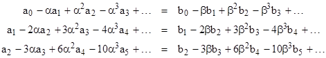
where the b_j are complex coefficients. In order for these two power series to be equal for arbitrary values of z in this region, we must equate the coefficients of powers of z, so we must have

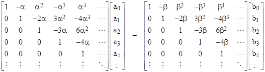
In matrix form these conditions can be written as

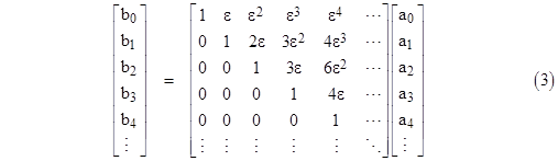
Multiplying through by the inverse of the right-hand coefficient matrix, this gives

where ε = β – α. Naturally this is equivalent to applying Taylor’s expansion. Now, it might seem as if this precludes any extension of the domain of the original power series. For example, suppose the original function was the power series for 1/(1 – z) about the point α = 0, so the power series coefficients a₀, a₁, … would all equal 1. According to the above matrix equation the coefficient b₀ for the power series about the point β would be simply

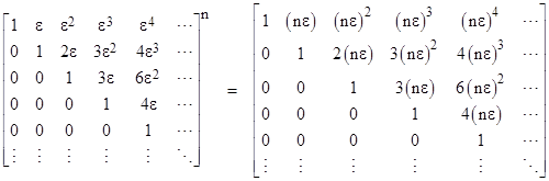
which of course converges only over the same region as the original power series. Also, it’s of no help to split up the series transformation into smaller steps, because the compositions of the coefficient matrix are given by

Thus the net effect of splitting ε into n segments of size ε/n and applying the individual transformation n times is evidently identical to the effect of performing the transformation in a single step. From this we might conclude that it’s impossible to analytically continue the power series 1 + z + z² + … to any point such as 3i/2 with magnitude greater than 1. However, it actually is possible to analytically continue the geometric series, but only because of conditional convergence.

This is most easily explained with an example. Beginning with the power series

centered on the origin, we can certainly express this as a power series centered on the complex number ε = 3i/4, because the power series f(z) and it derivatives are all convergent at this point (since it is inside the unit circle of convergence). By equation (3) with a₀ = a₁ = a₂ = … = 1, the coefficients of

are

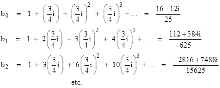
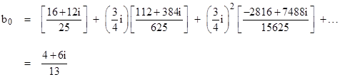
The absolute values of these coefficients are b_n = (4/5)ⁿ⁺¹. Now if we take these as the a_n values and apply the same transformation again, shifting the center of the power series by another ε = 3i/4, so that the resulting series is centered on 3i/2, we find that the zeroth coefficient given by equation (3) is

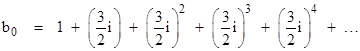
in agreement with the analytic expression for the function. This series clearly converges, because each term has geometrically decreasing magnitude. Similarly we can compute the higher order coefficients for the power series centered on the point 3i/2, which is well outside the radius of convergence of the original geometric series centered on the origin. But how can this be? We’ve essentially just multiplied the unit column vector by the coefficient vector for ε twice, which we know gives the divergent result

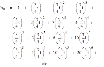
To examine this more closely, let us expand the quantities in the square brackets in the preceding expression for b₀. This gives

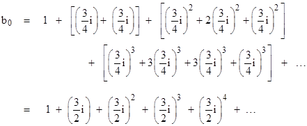
Each individual row is convergent, and moreover the rows converge on geometrically decreasing values, so the sum of the sums of the rows is also convergent. However, if we sum the individual values by diagonals we get

Thus the terms for b₀ are divergent if we sum them diagonally, but they are convergent if we sum them by rows. In other words, the series is conditionally convergent, which is to say, the sum of the series – and even whether it sums to a finite value at all – depends on the order in which we sum the terms. The same applies to the series for the other coefficients.

Since the terms of a conditionally convergent series can be re-arranged to give any value we choose, one might wonder if analytic continuation – which is based so fundamentally on conditional convergence – really gives a unique result. The answer is yes, but only because we carefully stipulate the procedure for transforming the power series coefficients in such a way as to cause the sums to be evaluated “by rows” and not in any other way. This procedure is justified mainly by the fact that it gives results that agree with the explicit analytic functions in cases when those functions are known.

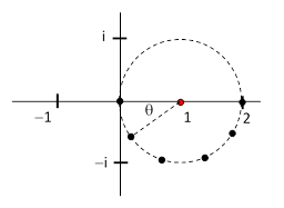
To show that we can also continue the geometric series to points on the other side of the singularity using this procedure, consider again the initial power series (4), and this time suppose we determine the sequence of series centered on points located along the unit circle centered on the point z = 1 as indicated in the figure below.

Thus, letting α = e^iθ, we wish to carry out successive shifts of the power series center by the increments

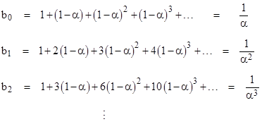
and so on. Applying equation (3) with ε = ε₁ to perform the first of these transformations we get the sequence of coefficients

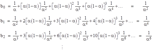
Now if we call these the a_j coefficients, and perform the next transformation using equation (3) with ε = ε₂, we get

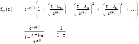
Each of these sums is clearly convergent, because |α| = 1 and |1-α| < 1. Continuing in this way, the nth power series in this sequence is

where m_n = (1 – e^niθ) is the nth point around the circle. This can also be written in the form

These examples demonstrate that equation (3) can be used consistently to give the analytic continuations of power series, although in cases where the sums cannot be explicitly identified by closed-form expressions there is a problem of sensitivity to the precision of the initial conditions and the subsequent computations. At each stage we need to evaluate infinite series, and the higher order coefficients tend to require more and more terms before they converge, and there are infinitely many coefficients to evaluate. If we limit our calculations to (say) just the first 1000 coefficients, the effect of the unspecified coefficients will propagate to c₀ in about 1000 steps. Smaller incremental steps require fewer terms for convergence of each sum, but they also require more transformations to reach any given point, and this necessitates carrying a larger number of coefficients. So, in practice, the pure numerical transformation of series using equation (3) often leads to difficulties. It’s also worth noting that many power series possess a “natural boundary”, i.e., the region of convergence is enclosed by a continuous locus of points at which the function is singular or not well-behaved in some other sense (e.g., not differentiable), and this prevents analytic continuation of the series. (See the note on The Roots of p.) Nevertheless, it’s interesting that an analytic function can, at least formally, be represented by a field of infinite-dimensional complex vectors, and that the process of analytic continuation can be represented by non-associative matrix multiplication. The failure of associativity is due to the fact that the convergence of the conditionally convergent series depends on the order in which we add the terms, and this depends on the order in which the matrix multiplications are performed.

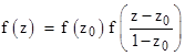
Incidentally, in each when analytically continuing the geometric series f(z) = 1 + z + z² + z³ + … by the procedure described above, we could have noted that the transformed functions centered on the point z₀ are expressible in the form

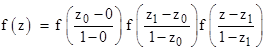
This is a simple functional equation, and it can be applied recursively to give the analytic continuation of the function to all points on the complex plane (except for the pole at z = 1). For any z we can choose a value of z₀ that is close enough to z so that the absolute value of (z-z₀)/(1-z₀) is less than 1 and hence the function f of that value converges. Of course, to apply the above equation we must also be able to evaluate f(z₀), even if the magnitude of z₀ exceeds 1, but we can do this by applying the formula again. For example, if we wish to evaluate f(3i) we could use the power series centered on z₁ = 7i/4, which requires us to evaluate f(7i/4), and this can be done using the power series centered on z₀ = 3i/4. Thus we can write

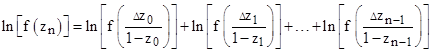
The argument of each of the right-hand functions has magnitude less than 1, so they can each be evaluated using the original geometric series to give f(3i) = 0.1 + 0.3i, which naturally agrees with the value 1/(1-3i). In general, to evaluate f(z_n) for any arbitrary value of z_n, we could split up a path from the origin to z_n into n small increments Dz and then multiply together the values of f(Δz/(1-z)) to give the overall result. If we take the natural log of both sides, the expression could be written in the form

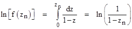
In the limit as the increments become arbitrarily small we can replace Δz with dz and integrate the right hand side. In this limiting case only the first-order term of the geometric series is significant, so we have

Therefore the integral of the right hand side reduces to

from which it follows (as we would expect) that

Another important aspect of analytic continuation is the fact that the continuation of a given power series to some point outside the original region of convergence can lead to different values depending on the path taken. This phenomenon didn’t arise in our previous examples, because the analytic function 1/(1-z) is single-valued over the entire complex plain, but some functions are found to be multi-valued when analytically continued. To illustrate, consider the power series

which of course equals ln(z) within the region of convergence. This series is centered about the point z = 1, and at z = 0 it yields the negative of the harmonic series, which diverges, so the function is singular at z = 0. Now suppose we analytically continue this power series to a sequence of power series centered on points on the unit circle around the origin, i.e., the sequence of points e^iθ, e^2iθ, e^3iθ, … for some constant angle θ.  Noting that the nth derivative of ln(z) is

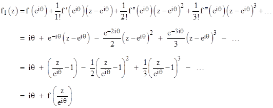
we see that the power series centered on the point e^iθ is given by the Taylor series expansion

Repeating this calculation for each successive point, we find

This converges provided |z–e^niθ| < 1. For nθ = 2πk we have f_n(z) = (2πi)k + f(z), so each time we circle the singularity at the origin the value of the function increases by 2πi. This is consistent with the fact that the natural log function (i.e., the inverse of the exponential function) of any given complex number has infinitely many values, separated by 2πi.

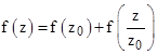
Notice that, in this case, our “functional equation” is simply

which can be used in a way analogous to how the functional equation for the geometric series was used to analytically continue the power series to all non-singular points. In this regard, it’s interesting to recall that the matrix formulation given by equation (3) is entirely generic, and applies to all power series, represented as infinite dimensional vectors, so whether or not a certain power series continues to a single-valued function (like the geometric series), a multi-valued function (like the series for the natural log), or can’t be continued at all, depends entirely on the initial “vector”.

Return to MathPages Main Menu