|
Variations on St. Petersburg |
|
|
|
And he dreamed, and behold a ladder was set up on earth, and the top of it reached to heaven, and behold the angels of God were ascending and descending on it! |
|
Genesis 28:12 |
|
|
|
Suppose someone owes us a dollar, and he offers us the following proposition: He will toss a fair coin, and if the coin comes up heads, his debt will be doubled, but if it comes up tails his debt will be cut in half. Should we accept this offer? |
|
|
|
The usual way of answering a question like this is in terms of the expected value. Since the debtor will owe us either 2 dollars or 1/2 dollar, each with probability 0.5, the expected value of the offer is 0.5(2) + 0.5(1/2) = 5/4 dollars. Thus the expected value increases by a factor of 5/4, so we may be inclined to accept the offer. If we were owed one dollar by each of a thousand people, and we made the same deal with each of them, we could be fairly confident of coming out ahead, because it’s very probable that roughly 500 would come up heads and 500 would come up tails, so our assets would increase by a factor of about 5/4. In order for us to lose money, the tails would need to exceed the heads by more than 2:1 out of 1000 coin tosses, which is extremely unlikely. On the other hand, it’s worth noting that with just a single debtor the risk is fairly high, because we have a 0.5 probability of losing half of our value. |
|
|
|
Now suppose the debtor alters his proposition. Instead of tossing the coin just once, he offers to toss it twice, and his debt will be doubled for each head (H) and cut in half for each tail (T). There are four equally probable outcomes for these two coin tosses. If the results are TT he will owe us only 1/4 dollar. If the results are TH or HT he will owe us 1 dollar. If the results are HH he will owe us 4 dollars. The expected value is therefore 0.25(1/4) + 0.25(1) + 0.25(1) + 0.25(4) = 25/16 dollars. Thus our expected value increases by a factor of 25/16, which is (5/4)2. |
|
|
|
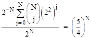
Similarly it’s easy to see that if the debtor offers to toss the coin N times, doubling the debt with each head and halving the debt with each tail, the expected value is |
|
|
|
|
|
|
|
Thus our expected value increased by a factor of 5/4 with each toss of the coin, so it would seem that it’s to our advantage to continue tossing the coin indefinitely, causing our expected value to rise without limit. |
|
|
|
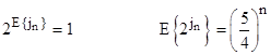
However, there’s another way of looking at this situation. Notice that we are always owed 2j dollars, and with each toss we either increase or decrease the exponent j by 1. For example, we begin with 20 dollars, and after the first toss we have either 2−1 or 2+1 dollars. In general, letting jn denote the exponent after the nth toss, we have jn+1 = jn ± 1. Thus the exponents can be modeled as a simple discrete random walk in one dimension. The expected value of the exponent after the first toss is 0.5(−1) + 0.5(+1) = 0, and likewise the expected value of the exponent remains zero after any number of tosses. In other words, letting E{x} denote the expected value of x, we have E{jn} = 0 for all n, and therefore we have the two interesting facts |
|
|
|
|
|
|
|
For example, with n = 1000 the expected value of jn is zero, corresponding to a debt of just 1 dollar, but the expected value of the debt is (5/4)1000, which is greater than 1096 dollars. |
|
|
|
Recall our previous scenario with 1000 debtors who each initially owed us a dollar, and they each tossed a coin to either double or halve their debt. We noted that the most likely outcome is 500 heads and 500 tails, which would increase our value by a factor of 5/4, from $1000 to $1250. This gain is quite robust, because the probability of the coin toss results differing enough from 500/500 to significantly reduce our gain is extremely small. The distribution of the number of heads has a mean of 500 with a standard deviation of about 16, so the 3-sigma case gives us 99.87% confidence of getting at least 452 heads, which still gives us $1178. In order to lose money overall, the coin tosses would need to yield only 333 heads (and 667 tails), which is about 10.4 standard deviations away from the mean outcome, with a probability of about 10−25. |
|
|
|
In contrast, if we have a single debtor who initially owes us $1, and he tosses a coin 1000 times and gets 500 heads and 500 tails (which is the single most likely outcome), he will still owe us exactly $1. Furthermore, the probability of losing money is 0.5. In fact, with a probability of almost 16% (the “1-sigma” case) we would end up with less than 2-16 dollars, meaning we would lose essentially all our money, despite the fact that the expected value of this arrangement is (as noted above) 1096 dollars. |
|
|
|
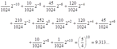
Furthermore, if we allow our debtor to continue tossing the coin indefinitely, the exponent j in the value of our asset, following a discrete random walk in one dimension, will eventually take on every finite value, and will do so infinitely many times. (See the note on The Gambler’s Ruin for an explanation of this.) Thus, no matter how high the value of the debt rises, it is always going to drop again down to microscopic amounts – after which it is going to rise to even greater heights, and so on. No amount of gain or loss is ever consolidated or secure in this process. If we consider the scenario in which the debtor agrees to toss the coin 10 times, there are 210 distinct possible sequences of heads and tails, and the expected value can be expressed explicitly as |
|
|
|
|
|
|
|
Much of the expected value comes from the least probable outcomes. We intuitively expect that, out of 10 coin tosses, the number of heads would likely be in the range from (say) 3 to 7. Indeed the probability of this is about 89%. If we focus on just the terms corresponding to those outcomes, the expected value is only 3 dollars, rather than 9.3 dollars. |
|
|
|
This illustrates the fact that a single “expected value” doesn’t provide a complete characterization of our meaningful expectations. For example, if there were a process that automatically increased our value by a factor of 5/4 on each round, the expected value of n rounds would be (5/4)n, just as it is in our double-or-halve scenario, and yet our expectations have quite a different character in these two scenarios. In the automatic case our value is certain to equal (5/4)n after n rounds, whereas in our double-or-halve scenario it is almost certain to be much less. Also, in the automatic case we can never lose money, whereas in the double-or-halve scenario we have a 50% chance of losing money. Clearly the “expected value” doesn’t tell the whole story – even if we naively equate each numerical amount of money with utility, which is often unrealistic, especially with exponentially varying values. (For a closely related discussion, see the article on the Two Envelopes.) |
|
|
|
The same issues arises when considering the St. Petersburg paradox. Someone offers to toss a fair coin until it comes up tails. If the first tails occurs on the nth toss, they will give us 2n dollars. How much would we pay to play this game? The probability of winning k dollars is 1/2k, so we have a 50% chance of winning just 1 dollar, a 25% chance of winning 2 dollars, and so on. The expected value is infinite, and yet most people would not be willing to pay more than (say) $20 to play this game. This is because we recognize that most of the expectation comes from extremely improbable (not to mention unrealistic) outcomes. If we disregard the outcomes that involve more than 20 heads in row, the expected value is only $20. The question of realistic utility is also important, since we can’t realistically expect to collect, say, 2100 dollars, nor would such an amount have any realistic utility, since it far exceeds the value of everything that can be bought. |
|
|
|
Incidentally, when reviewing attempts to apply probabilistic reasoning to real world situations, we often find that people unconsciously establish hierarchies, splitting the problem into multiple levels, albeit sometimes in ways that don’t make sense. For example, when trying to show that the catastrophic failure of a certain system has probability less than 10−9, people sometimes analyze the system only under certain conditions, justifying this by pointing out that the system operates in those conditions 99.9% of the time. On this basis, they assert that the probability of failure is probably 10−9, neglecting the other 0.1% of conditions. Of course, this is ridiculous, since if the system is certain to fail catastrophically when operating in the 0.1% of conditions not covered by this analysis, the overall probability of catastrophic failure is 10−1, not 10−9. This is an example of an invalid hierarchy. In a valid use of hierarchy, the probability of failing the conditional must obviously be smaller than the probability of the system failure that we are trying to calculate. |
|
|
|
It’s interesting to compare the two different wagering propositions discussed above with the two types of evolution of the wave function in ordinary quantum mechanics. The scenario in which we begin with one dollar of debt, and then simple toss the coin repeatedly, without ever consolidating our gain (or loss) at any point, is somewhat analogous to the unitary evolution of the wave function under the Schrodinger equation. The wave function evolves into a superposition of all possible outcomes, much like all the possible values of 2j in our random walk on the exponent j. In this process we just “let it ride” repeatedly, and this is (in a sense) a reversible process, since the exponent will take on the same range of values when evolving either forward or backwards. (In either direction, the exponent has an equal probability of incrementing or decrementing by 1 on each step.) At the other extreme, we could loan someone a dollar, toss the coin just once, take our gain or loss, and then repeat this process over and over (loaning him a dollar each time). In this scenario the evolution of the situation is quite different, as we will gradually consolidate the expected gain, and this is not a reversible process. This is somewhat analogous to the irreversible measurement process in quantum mechanics, by which the wave function “collapses” on a particular outcome, consolidating the gain or loss irreversibly. |
|
|