A Trigonometric Path to Basel

Two of the best known elementary trigonometric identities are

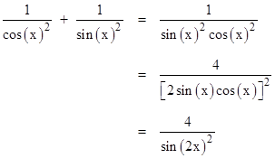
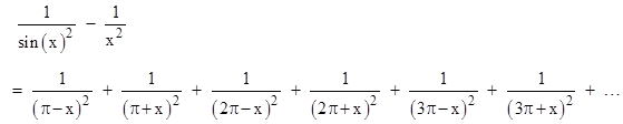
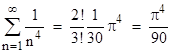
From these we can deduce the solution of the so-called Basel problem, which is to find the sum of the squared reciprocals of the natural numbers (first solved by Euler by a different method). Dividing through by the squared product of the sine and cosine, the sum of squares identity can be re-written as

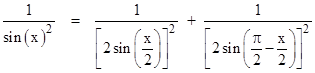
Making use of the fact that cos(x) = sin(π/2 − x), and replacing x with x/2, this gives the identity

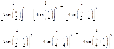
Applying this same identity, the two terms on the right side can be expressed as

The arguments of the sines on the right sides of these equations are

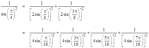
These quantities are in arithmetic progression just if x = π/4, in which case the arguments are

Thus we have the equalities

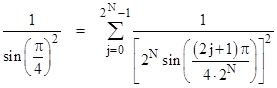
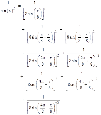
Iterating this process, we can expand each of the four terms in the last expression into two terms using the basic identity, to arrive at an equivalent sum of eight terms with the sine arguments kπ/32 where k = 1, 3, 5, …, 15. And so on. In general, for any positive integer N, we have

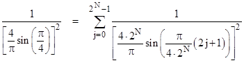
Dividing through both sides of this equality by (4/π)² we get

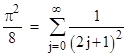
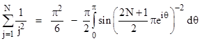
Each time we increment N, the number of terms on the right side doubles, and the denominator of the sine arguments doubles, so the (arbitrary number of) initial arguments become arbitrarily small, and in this limit the sine approaches the argument. (As the arguments approach π/2 the sines are less than the arguments, so those contributions don’t interfere with convergence.) In the limit as N goes to infinity, and noting that the left side equals π²/8, we have

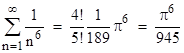
This is the sum of the squared reciprocals of the odd natural numbers, which we can denote as S_odd, and we seek the sum S of the squared reciprocals of all the natural numbers, which is given by S = S_odd + S_even where S_even is the sum of the reciprocals of the even natural numbers. It’s easy to see that S_even = S/4, so we have S = (4/3)S_odd, and hence S = π²/6 as was to be shown.

This approach also leads to a more general identity. Instead of specializing to x = π/4, we can allow x to be an arbitrary quantity, and we have at the third level

Bringing the leading term on the right side over to the left, and proceeding on to the kth level for N=2^k , the arguments of the leading sines become arbitrarily small, so we have the limiting relation as N → ∞

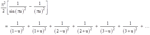
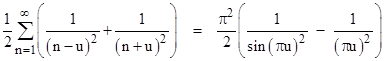
When x is any multiple of π, one of the terms in the series is infinite, so the equality applies only for x in the range from 0 to π. In terms of a new parameter u defined by x = πu, we can multiply through by π² and get the relation (as N goes to infinity)

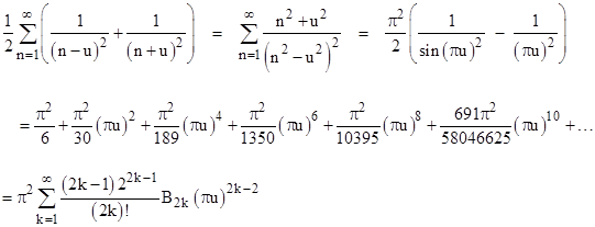
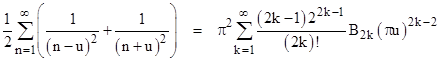
Thus we have

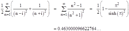
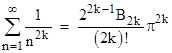
where B_2k are the (positive) Bernoulli numbers. With u=0 this gives the Basel sum, whereas if we take (for example) u = √-1 we have

Writing the preceding equation as

we can differentiate both sides with respect to u to give

Differentiating both sides again, we get

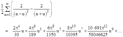
Putting u = 0, this gives the next of Euler’s results for even reciprocal powers

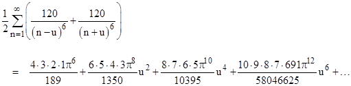
Differentiating the previous expression twice more gives

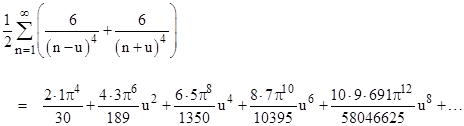
and evaluating this at u=0 we get the sum of the reciprocals of the 6^th powers

Thus for the general sum of reciprocals of the (2k)th powers, we have

As an aside, let us return to the relation

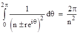
and recall that this series is valid for u between 0 and 1. Suppose we set u = re^iθ for some real magnitude r (with |r|<1) and phase θ, and integrate both sides from θ = 0 to 2π. Thus we are integrating around a circle of radius r centered on the origin of the complex plane. In view of the integral

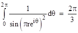
we can integrate the left side of the previous equation term-by-term to give π³/3, independent of r. Therefore, the integral of the right side of that equation must also equal this value, independent of r (provided |r| < 1). The integral of the second term in that expression is zero, so we have

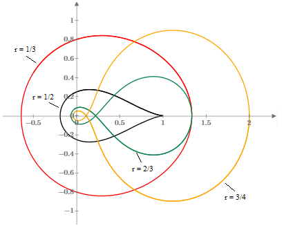
This is slightly non-trivial, because the integrand function has both real and complex parts, and traces out a variety of loci in the complex plane for various values of r, as shown below.

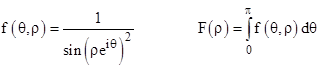
Despite the variety of these loci, the imaginary part of the integral always vanishes (because they are symmetrical about the real axis) and the real part always equals 2π/3. This plot somewhat disguises things because it doesn’t show the variation in density as a function of θ. To clarify, let us define the function

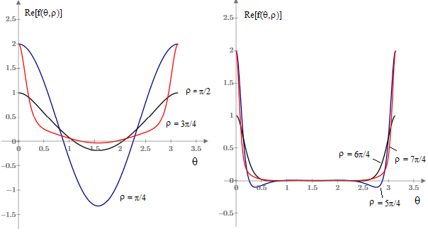
Thus F(ρ) is the integral of 1/sin(z)² as z traces out an upper half circle of radius ρ in the complex plane. The plot on the left below shows f(θ,ρ) for three values of ρ in the range from 0 to π. The integrals F(ρ) of these three functions are each equal to π/3.

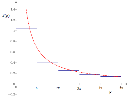
In fact, we have F(ρ) = π/3 = 1.04719… for every real ρ in the range from 0 to π. However, for values of ρ in the range from π to 2π we have F(ρ) = 0.410577… as exemplified by the curves in the right hand plot above. For values of ρ in the range from 2π to 3π we have F(ρ) = 0.251422…, and so on. A plot of F(ρ) is shown below.

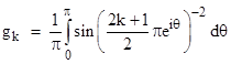
The dashed line represents 0.675/ρ, which shows that the discrete values decrease in inverse proportion to ρ. To determine the exact values, let us define the values of the normalized integral for each of the ranges by setting ρ to the mid-point of the range (for convenience), so we have the quantities:

Thus we have g₀ = 1/3, g₁ = 0.1306909660…, g₂ = 0.080030374…, and so on. Now we notice that the differences (g₀ – g₁), (g₁ – g₂), (g₂ – g₃), … are in the proportion 1, 1/4, 1/9, and so on. From this it follows that for any N we have

In the limit as N approaches infinity the value of g_N goes to zero and the summation of reciprocal squares goes to π²/6, so we have

Therefore, since g₀ = 1/3, we have for N > 0

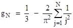
Solving this for the partial sums of reciprocal squares and inserting the expression for g_N, we have

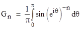
Instead of considering just the squared reciprocal sines, we can consider the more general functions involving the nth power of the reciprocal sines (and normalizing the integral for convenience), and we can focus on a value of ρ (such as 1) in the principle range 0 to π . This leads us to define

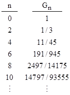
which has the rational values (for even n)

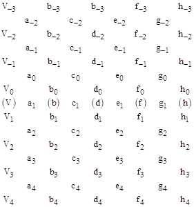
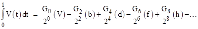
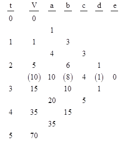
Interestingly, these coefficients have an application in the Gauss-Encke numerical integration formula. Given a sequence of equally-spaced discrete values V_j = V(j), j = …−3, −2, …, 3, 4, … of a continuous analytic function V(t) separated by units of the ordinate t, we can form the first differences a_j = V_j – V_j−1, and the second differences b_j = a_j+1 – a_j, and so on, as depicted in the array below.

We then define the central means (V) = (V₀ + V₁)/2, and (b) = (b₀ + b₁)/2, and so on. Then the Gauss-Encke estimate of the integral of the function V(t) from t = 0 to 1 is given by

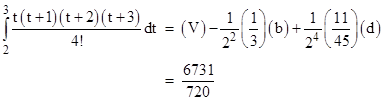
For example, with V(t) = t(t−1)/2 we have the values 0, 1, 3, 6, 10, 15, …, with the first differences 1, 2, 3, 4, 5, …, and the second differences 1, 1, 1, 1, …  All higher-order differences are zero. Therefore, since G₂/2² = 1/12 and (b) = 1, the integral of V(t) between any two consecutive values is the average of those values minus 1/12. For another example, with the function

we have the values and differences

so we have (V) = 10, (b) = 8, and (d) = 1, and all higher order differences are zero. We can use the integration formula to compute

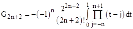
The usual way of computing the even-indexed G_n coefficients is by the rational integral

although the equivalence between this integral of rational functions and the previous integral of transcendental functions seems non-trivial.

Return to MathPages Main Menu