Reliability with Periodic Repairs

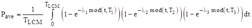
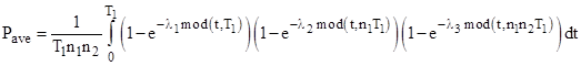
Consider a system with N=3 components with exponential failure rates λ₁, λ₂, λ₃, and suppose they can fail latently and they are inspected (and repaired) every T₁, T₂, and T₃ hours respectively. These inspection cycles are assumed to originally begin simultaneously, and thereafter the entire cycle repeats every T_LCM hours, where T_LCM is the least common multiple of T₁, T₂, and T₃. The average probability of being failed can be formally expressed as

where mod(x,y) is the remainder of x when divided by y, meaning the amount by which x exceeds the next lowest whole multiple of y. To evaluate this integral numerically, care must be taken to use sufficient precision, since the function is discontinuous at each repair time.

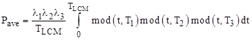
If all the values of λ_jT_j are always orders of magnitude smaller than 1, the above expression can be simplified to

in which case the problem reduces to evaluating the average value of the product of sawtooth functions, as discussed in another note for the case of nested intervals, i.e., when n₁ = T₂/T₁ and n₂ = T₃/T₂ are integers. In that case we have T_LCM = T₃ = n₁n₂T₁, and we can express P_ave as an integral with t ranging from 0 to just T₁, taking as the integrand the following triple summation:

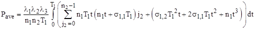
The summand can be expanded as

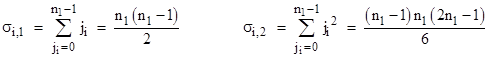
So, using the sums of powers identities

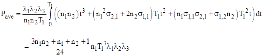
we can evaluate the inner summation and write the expression for P_ave as

Evaluating the remaining summation, we get

Recalling that, for small λT, the maximum probability is

we have the result

This agrees with the result derived in the article on products of sawtooth functions. The above is merely more explicit about the summations involved in the integrand.

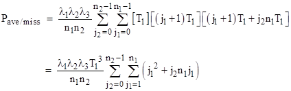
Incidentally, the literature contains a treatment of this subject that regards the shortest interval T₁ as a single mission, and deals with the average “per mission” probability by assigning the probability at the end of each of those short intervals to the entire interval. Hence there is no integration, and the value of t in the integrand of equation (1) is replaced with T₁, resulting in

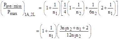
Evaluating the summations using the sum-of-powers identities noted above, and dividing through by P_max, the quoted result in the literature is

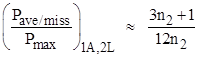
This is typically presented as a result applicable to systems with one active and two latent faults, and there is no averaging for the probability of the active fault during the mission (T₁) interval, explaining why this is larger by about a factor of 2 relative to equation (2). Also note that n₁, the number of missions in the shortest inspection interval, is typically at least 10 and possibly 100 or more, whereas n₂ is typically not too large, so this expression is asymptotic to

which is just the ratio of N=2 latent faults. This is as expected, because the active fault is being exempted from averaging, so it is separate from the two latent faults, which can be analyzed separately. The resulting equation is not to be confused with a true averaging of three faults given by equation (2).

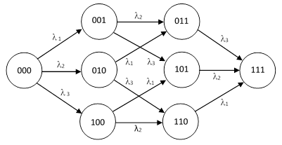
The first equation at the beginning of this article is exact for all values of λT, not just for values much less than 1, whereas the subsequent formulas were developed under the “λT << 1” assumption. Another approach that is exact for all conditions is to use a Markov model with periodic repair transitions. To illustrate, consider again a system with three components, for which the model with no repairs is as shown below.

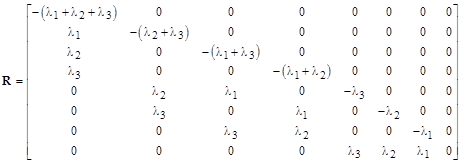
The failure transition matrix is

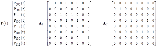
The state vector and the transition matrices for repairing component 1 and component 2 respectively are

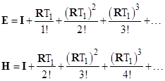
We don’t need to repair transition matrix for component 3, because that repair occurs at the end of the overall cycle, and we are evaluating the average probability only over one cycle. We now define the exponential and integrated exponential functions matrices, which are most easily computed by the series

where it is typically sufficient to include just the first six terms or so for high precision. Then we have

where P(0) is the initial state with all the probability in the full-up state, i.e., the column vector transpose of [1,0,0,0,0,0,00]. The value of the last element of P_ave is the average probability of “State 111”, i.e., the state in which all three components are failed. This should agree exactly with the value of

To illustrate this, consider the case λ₁ = λ₂ = 0.0001/hour, λ₃ = 0.00001/hour, n₁ = 3, n₂ = 4, T₁ = 100 hours. Both of these equations give the probability (5.39872809)10⁻⁷. To reach this precision of agreement it’s necessary to evaluate the exponential matrix to the 6^th degree, and to use high precision to evaluate the integral (since it contains discontinuities). The maximum probability can easily be computed as

and the approximate value of P_ave/P_max given by equation (2) for our example is 0.152778, so we would approximate P_ave by (5.359098)10⁻⁷, which differs from the exact value by just 0.73%.

The H matrix in equation (3) represents the average probability over the time period T₁, but suppose T₁ consists of n₀ missions of duration T₁/n₀, and we want the average of the mission probabilities, with an exposure time of an entire mission. In that case we replace H with the corresponding average of discrete probabilities. For that purpose, let us define the matrices

In these terms the discretized equation can be written as

The first factor on the right side asymptotically approaches H as n₀ increases. The summation limits in the first factor are incremented by 1 because we are assigning to each sub-interval the probability at the end (not the beginning) of the interval.

Return to MathPages Main Menu