Time and Distance for Dual Motors

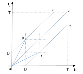
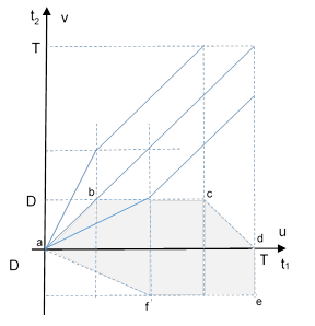
Further to the note on Dual Failures with General Densities, consider a twin-motor vehicle that carries out missions of duration T hours, with a maximum diversion time of D hours if one of the motors fails. Each motor has an independent failure density function δ(t). We begin by assuming that the vehicle speed is essentially the same whether it is operating with both motors or just one. (Later we will determine the effect of a reduced speed during single-motor operation.) If the first motor failure occurs less then D hours after departure, the vehicle will return to its point of departure. If the first motor failure occurs less than D hours from the destination, the vehicle will continue to its destination. Based on these premises, the probability of both motors failing during a mission attempt is given by the integral over the relevant region of the joint probability function δ(t₁)δ(t₂) where t₁ and t₂ are the times to the next failures of the motors at departure. The relevant region is shown in the figure below.

The dual failure during a mission occurs just if (t₁,t₂) falls within the region enclosed by abcdefa. To integrate the joint density function over this region it’s convenient to work with the rotated coordinates defined by

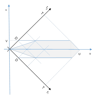
The determinant of this transformation is unity, so we have du dv = dt₁ dt₂. The rotated version of the drawing is shown below.

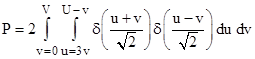
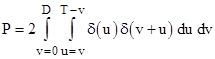
The shaded region is symmetrical for positive and negative v, so we can just take twice the integral of the positive v region. Thus the probability is given by

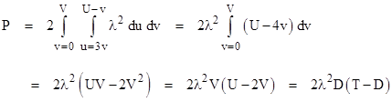
where U = T√2 and V = D/√2. For example, in the simple case with essentially constant failure density δ(t) = λ, we get for D < T/2 the result

A slightly less intuitive but more efficient transformation, leading to the same results, is given by t₁ = u and t₂ = u+v, which has the inverse transformation u = t₁ and v = t₂ – t₁. The determinant of this transformation is unity, so it (again) preserves areas, but this isn’t a conformal map (i.e., it doesn’t preserve angles or shapes), it is a laminar transformation. It essentially slides each vertical slice downward such that the main diagonal is mapped to the horizontal axis, as shown in the figure below.

The vertices of the original region are mapped to abcdef on this plot, and it’s easy to see that the area under the u axis is equal to the area above the u axis (even though the mapped shapes are different), so we need only compute twice the integral of the upper region. Thus we have

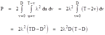
As before we consider the simple case δ(t) = λ, which now gives

in agreement with the previous result.

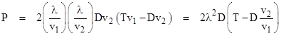
To this point we have focused on the case of a vehicle with constant speed, regardless of whether one of the motors is failed. For this case the time intervals are proportional to the distance intervals. However, we can also consider the case where the vehicle moves at speed v₁ with both motors running, but it moves at a slower speed v₂ when one motor has failed. In this case we cannot simply treat distances as being proportional to time intervals. For example, if the vehicle is just one hour from its destination, assuming speed v₁, and an motor fails at this point, causing the speed to be reduced to v₂, the vehicle will take more than one hour to reach its destination, which shows that the total mission length can exceed T in this case. Still, the total distance traveled would never exceed Tv₁, and the diversion distance will not exceed Dv₂. To take this into account we can repeat the calculation shown above, but on a distance basis rather than a time basis, using Tv₁ in place of T, and using Dv₂ in place of D. Also, we must account for the fact that the failure density λ (in the example above) is expressed as failures per unit time, so we need to use a rate expressed as failures per unit distance, which implies that the rate (on a distance basis) is greater during single-motor diversion (because of the lower speed) than during normal two-motor operation. Thus for normal operation we replace λ with λ/v₁, and for the diversion we replace λ with λ/v₂. Making these substitutions, we get

This applies provided v₂D < v₁T/2.

Return to MathPages Main Menu