|
Required Order Factors |
|
|
|
Where there is no law, there is the least of real liberty. |
|
Henry Martyn Robert |
|
|
|
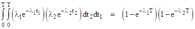
The probability that two independent components with constant failure rates λ1 and λ2 will both fail during a time interval T is |
|
|
|
|
|
|
|
where t1 and t2 are the times when the respective components fail during the interval. If the values of λjT are both orders of magnitude smaller than 1, the above expression is closely approximated by (λ1T)(λ2T). This integral represents the fact that each component can fail at any time during the interval from 0 to T. |
|
|
|
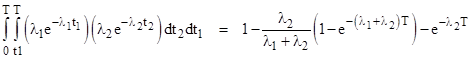
In some circumstances we are interested in the probability that the two components will fail during a given interval in a specific order. To compute that probability, we can simply integrate the joint density over the region that satisfies the required order. For example, if we want to know the probability that both components fail and component 1 fails before component 2, we evaluate the integral as follows |
|
|
|
|
|
|
|
If λ1T and λ2T are both orders of magnitude smaller than 1, this reduces to (1/2)(λ1T)(λ2T), so in this case the probability of both components failing in the specified order during the interval is 1/2 times the unordered probability. This is sometimes called a Required Order Factor (ROF), and is often applied to the basic probability in a fault tree to take credit for the required order. It’s worth emphasizing that the simple approximation of 1/2 for the case of two components failing in a specific order is valid even for unequal failure rates, provided only that the values of λ1T and λ2T are small, because in that limit the density distribution for each failure is uniform over the interval, so each component is equally likely to fail at any time during that interval. Hence each permutation of the sequence of failures is equally probable. |
|
|
|
More generally, for any specified order requirements on a set of n components failing within an interval of time T, there are n! possible permutations of these components, corresponding to the n! possible sequences of failure, and if we let k denote the number of permutations that satisfy the order requirements, then the required order factor is closely approximated by k/n!, provided the probabilities are all sufficiently small. |
|
|
|
However, if the probabilities are greater than about 0.01, the simple combinatorial approximation becomes inaccurate, because the permutations are not all equally probable. In that case the exact integral, as in the example above, must be used. As an example, suppose a fault tree has a cutset with five components, denoted by C1 to C5, and suppose that were are interested in the probability that they all fail in the interval T, and that the component C1 fails after C3 and C4, and that the component C2 fails after C3, C4, and C5. If all the probabilities are small, we can use the simple combinatorial approach and simply count how many of the 5! = 120 permutations satisfy the specified order conditions. There are 6 permutations of C3, C4, C5, and we know C2 must occur after those three, and C1 must occur either after those three as well, in which case there are two permutations of C1 and C2, or between the second and third of the first three if the last of those is C5, so there are just two of those (permuting C3 and C4). Thus there are 6∙2 + 2∙1 = 14 permutation that satisfy the specified order requirements, and hence the ROF is 14/120 = 0.117. |
|
|
|
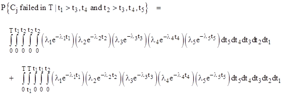
As noted, the combinatorial approximation is valid only if the probabilities are sufficiently small. If the probabilities are large, we must integrate the joint density function exactly. To integrate over the required regions, we form two quintuple-nested integrals, one with t1 ranging from 0 to T and with t2 ranging from 0 to t1, and the other with t1 (again) ranging from 0 to T and with t2 ranging from t1 to T. In the first case, t3, t4, and t5 each range from 0 to t2, and in the second case they range from 0 to t1, t1, and t2 respectively. Thus the probability of these five faults occurring in an order the satisfies the specified requirements is the sum of the two integrals: |
|
|
|
|
|
|
|
Dividing this sum by the quantity |
|
|
|
|
|
|
|
gives the ROF for this cutset. With λ1 = λ2 = 10−5 and λ3 = λ4 = λ5 = 10−6 and T=1000 hours the probabilities are not too large, and this gives the factor 0.116, fairly close to the simple combinatoric factor. However, with T=50,000 hours the probabilities of C1 and C2 are 0.393 and the probabilities of C3, C4, and C5 are 0.049, so we expect a smaller ROF because the components that need to fail later are more likely to fail sooner in the interval. For this case we get the required order factor 0.093. On the other hand, with λ1 = λ2 = 10−6 and λ3 = λ4 = λ5 = 10−5 and T=50,000 hours the components that need to fail last are more likely to fail later in the interval, so for this case we get the required order factor 0.144. |
|
|