The Failure Rate Function

Do not infest your mind with beating on

The strangeness of this business; at pick'd leisure

Which shall be shortly, single I'll resolve you,

Which to you shall seem probable, of every

These happen'd accidents; till when, be cheerful

And think of each thing well.

                                         Shakespeare

For any given (cumulative) probability distribution P(t) we can define the failure rate function h(t) as

(The symbol “h” is used for this function because it is sometimes called the hazard rate function.) For example, a simple “exponential” distribution P(t) = 1 – e^−λt for some constant λ has the failure rate function h(t) = λ. The definition (1) can be written in the form

which has the elementary solution

Thus we have

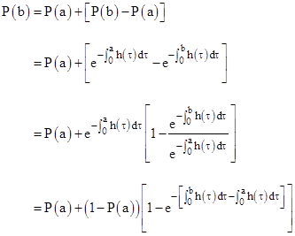
Given the value of P(t) at some specified time t = a, we can express the value at some later time t = b as

Thus we have

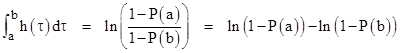
This applies to any arbitrary failure rate function, and it appears in published regulatory requirements for numerical safety calculations. Re-arranging terms, this can also be written in the form

If the probabilities are orders of magnitude smaller than 1, we can make use of the first-order term in the expansion ln(1−x) = −[x + x²/2 + x³/3 + …] to give the approximate relation

This confirms that the failure rate function is approximately equal to the probability density function for sufficiently small probabilities. Nevertheless, the two functions should not be conflated, especially for latent failure condition that may eventually acquire large probabilities.

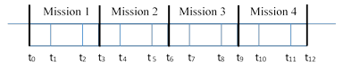
In some circumstances we may consider a sequence of missions, each consisting of a sequence of phases, possibly with different failure rate functions in each phase, and we may wish to determine the probability of an element being failed at the end of each mission. For example, if each mission consists of three phases, then a sequence of four missions could have a total time-line as depicted below.

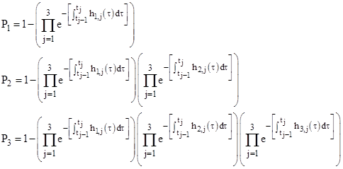
We can split the integrand of equation (2) into individual phase segments as follows:

Letting h_k,1(τ), h_k,2(τ), and h_k,3(τ) denote the rate function for the three phases on the kth mission, where τ is measured from the start of the respective mission, the probability P_k at the end of the kth mission can be written as

and so on. Letting q_k denote the product in parentheses, we can write these relations more succinctly as

and so on. Thus we have

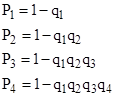
Restoring the full expression for q_k, and generalizing to n phases per mission, the probability at the end of the kth mission can be computed recursively by the formula

This recursive formulation enables us to compute the probabilities at the end of each mission, while aggregating the repeated sequence of phases within the missions. If the h_k,j failure rate functions are the same for all mission, then this is simply P_k = P_k−1 + (1−P_k−1)P₁ with P₀ = 0. Of course, if the element is checked (and, if necessary, repaired) prior to each mission, we set P_k−1 = 0 in (4).

As noted above, the simple exponential distribution P(t) = 1 – e^−λt for some constant λ has the failure rate function h(t) = λ, but the joint probability distribution

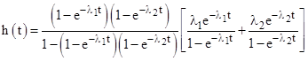
for constants λ₁ and λ₂, representing the probability that two independent and exponentially distributed components are both failed by time t, has the failure rate function

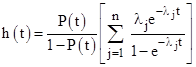
More generally, the joint probability distribution for the failure of n independent exponentially distributed components with constant failure rates λ_j is

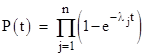
and the corresponding failure rate function is

It is perfectly possible to use these complete failure rate functions in equations (2) or (3), so we need not restrict ourselves to individual elements. Of course, whether we apply these equations to the joint rate function of the overall cutset, or to the individual elements and then take the product of the result, we get exactly the same result.

As an aside, published regulatory guidance calls for computing the probability of failure on each mission, then computing the simple arithmetical average of those mission probabilities, and then dividing this average by the standard mission duration. Interestingly, both of these seemingly simple steps have sometimes been regarded as controversial. The averaging step has been challenged because, for the cumulative probabilities of latent faults, the sum of the probabilities in the numerator of the average can exceed 1. Of course, this sum is not a probability, so there is nothing objectionable about it exceeding 1. For example, suppose the probability of rain on each of the five days (Monday to Friday) is 0.8, and someone defines the quantity called “Average Probability” as literally the arithmetical average of those probabilities, which gives

This result should not be surprising. Note that the numerator of the calculation, which has the value 4.0, is not a probability, it is an arithmetical sum of probabilities, and need  not be in the range 0 to 1. (It would be a probability only if the conditions were mutually exclusive, e.g., if it rains on Monday it can’t rain on Tuesday, but that is not the case, just as it is not the case that if a certain latent failure condition is present on Monday it can’t also be present on Tuesday. Nevertheless, the arithmetical average of a set of values in the range from 0 to 1 is also in that range.) Now, someone might argue that the numerator of this calculation shouldn’t be the sum of the probabilities (even though the regulations explicitly state that it is), it “ought to be” the probability of the “sum”, i.e., the union of the rain condition on the five days. According to this notion, the numerator of the calculation should be 1 – (1−0.8)⁵ = 0.99968, and hence the “Average Probability” of rain for those five days “ought to be” about 0.2. This isn’t a particularly useful definition of “average”.

The last step of the regulatory calculation (dividing by the average mission duration) is also sometimes debated. In this case the reason for the confusion is more understandable, because, in general, dividing a probability (or average of probabilities) by a time duration doesn’t yield a quantity with a natural meaning. It is neither a probability nor a failure rate, even though it has units of hour⁻¹. As in the above discussion, there are certainly meaningful quantities involving probability with these units, such as dP/dt, but clearly the derivative of probability doesn’t represent a valid measure of unreliability or risk. For example, if a system is permanently failed with probability 1, we have dP/dt = 0. On the other hand, people sometimes compute the probability of a component being failed by time T as 1 – e^−λT, and they imagine that this quantity divided by T represents the “probability per hour”. They associate this quantity with the failure rate λ, which it equals for sufficiently small values of λT, but of course for larger exposure times the probability asymptotically approaches 1, regardless of the failure rate, so a system with λ = 1/100 per hour, after operating for 100,000 hours, during almost all of which it was almost certainly failed, would have a “probability per hour” (according to this strange construal) of about 1/T, which is 1E-05/hr. If we increased the latency period to ten million hours, this same system would be assessed to have a “probability per hour” of 1E-07/hr, even though it is almost certainly failed for nearly its entire life. These numbers clearly bear no meaningful relation to the probability of the unit being failed.  In general, arithmetically dividing a probability at the end of an interval by the duration of the interval is “not a thing”.

What, then, is the purpose of dividing the (average) per-mission probability by the mission length in the regulatory guidance? Why not just impose numerical limits on the per-mission probability? The original purpose of this step was to account for differences in mission lengths for different products. To place the products on an equal footing of fatalities per passenger mile, it’s necessary to scale the per-mission probabilities by the average mission length for the product. This is a commonplace practice in many branches of engineering. For example, the rotor speed of a motor can be quoted as physical revolutions per minute (RPM), but the performance of the motor at different ambient temperatures can be normalized to a common basis if we divide the speed by the square root of the (absolute) temperature. Of course, if we do this, the resulting quantity has units of RPM/√°K, which would be confusing. To avoid the dimensional confusion resulting from this “correction”, it is typical to define the temperature correction factor θ = T/T₀, where T₀ is the temperature for some standard reference condition. The value of θ is dimensionless, and is used to defined normalized (aka corrected, referred) rotational speed parameters such as N1/√θ, which has ordinary units of RPM.

Likewise the regulatory authorities could have avoided generations of confusion by normalizing to some standard mission duration, such as T₀ = 1 hour, and requiring that the per-mission probabilities for models with mission duration T be divided by the dimensionless ratio T/T₀. This is obviously numerically equivalent to just dividing by T, but it eliminates the spurious units that lead to so much confusion. It should be kept in mind that a normalized probability is not a failure rate. The actual failure rate function, as defined above, has a perfectly clear meaning, and is used in the formulation of the regulatory guidance, but it is not to be confused with vague and ill-defined notions of “probabilities divided by exposure times”, and the variety of concepts that are elicited by the phrase “probability per hour”. Interestingly, over a period of decades, the original purpose and understanding of the formulated risk criteria can be lost, and entirely new interpretations (of varying levels of conceptual coherence) can be placed on it.

Return to MathPages Main Menu