Appendix A:  Discrete-Time Simulation of Feedback Loops

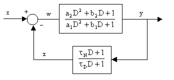
Consider two transfer functions arranged in a feedback loop as shown below

By the methods described in previous sections we can determine the following two recurrence formulas for the two individual transfer functions:

We also have the equation for the summing junction

Together these three formulas define the dynamic relationship between x_n and y_n. However, they cannot be executed as written, because the computation of y_i by equation (A1) requires the value of w_i, and the computation of w_i by equation (A3) requires the value of z_i, but the computation of z_i by equation (A2) requires the value of y_i, which is what we are trying to find.

A simple approach to simulating this system would be to approximate the summing junction equation by

In other words, w_i would be computed as the current value of x minus the past value of z. However, in some circumstances, especially when x changes rapidly, this approximation can lead to unrealistic and even unstable results.

To overcome this problem it is necessary to “solve” the complete set of loop equations simultaneously. We’ll first show how this is done for loops in which all the piece-wise relationships are linear functions (as in the preceding example), and then we will show how this approach can be modified to accommodate non-linear functions.

Assuming all the functions in the loop are linear, we re-write equation (A1) for y_i, and eliminate all appearances of w_i by substituting from equation (A3), which gives

The corresponding equation for y_i-1 is

Also, equation (A2) can be written for the times t_i-2, t_i-1, and t_i as follows

Equations (A5) through (A9) constitute five equations in the five unknowns z_i-3, z_i-2, z_i-1, z_i, and y_i. Solving these equations simultaneously gives the following recurrence formula for y_i:

where

Now suppose the first-order lead/lag in the above example were replaced by an arbitrary function F of y, that is

Substituting this into equation (A5) and rearranging terms gives the equation

At each application of this (implicit) recurrence formula we are given the values of y_i-2, y_i-1, x_i-2, x_i-1, and x_i, so the right side of (A12) can be computed (assuming F is computable). Given this value, which we will denote as V_i, equation (A12) is simply

Depending on the form of the function F, this equation may or may not be explicitly solvable for y_i. In any case, it can be solved numerically to any desired degree of precision.

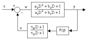
If the arbitrary function F is inserted into the feedback loop in series with (rather than in place of) the dynamic function, the resulting set of equations can still be reduced to essentially the same form as (A13). Consider the feedback loop shown below.

By substituting F(y_n) for y_n in equations (A7), (A8), and (A9), we can solve the five equations (A5) through (A9) for y_i to give

The right hand side of this equation consists entirely of “given” information. If we call the right hand value V_i then the recurrence formula is

As in the case of equation (A13), this equation may or may not be explicitly solvable for y_i, but a numerical solution of any desired precision can be computed. Notice that the execution frequency of the algorithm must be high enough so that the values of y_n occur close enough together so that the discrete values of F(y_n) provide an adequate definition of the actual function F(y(t)).

Return to Table of Contents