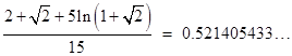
Distances In Bounded Regions

One of the standard problems in introductory calculus courses is to find the average distance between two randomly selected points inside a unit sphere.  The popularity of this particular problem is probably due to the fact that it happens to lead to an integral that can be evaluated in "closed form" to give a nice explicit answer, but it's interesting to consider the average distances (and powers of distances) within various other bounded regions in various dimensions.  For regions other than a sphere, the solution is not always so simple, but we'll find that a parametric formulation of the distance density can be used to simplify the analysis. 

We'll begin by considering circles (spheres) and squares (cubes) of different dimensions, starting with the classic problem of the solid unit sphere in 3D space.  Let R and r be the radial distances from the origin to two randomly chosen points in a unit sphere, and let θ be the angle between these vectors.  The distance between the two points is 

Covering just the case R > r, we need to triple-integrate this quantity over r, R, and θ, and we need to weight the quantity in proportion to the fraction of the two-point state-space corresponding to each set of parameters.  For given values of r and R, the angle θ defines a circle whose circumference is proportional to sin(θ), so this is the weight for the θ integration.  Similarly each value of r and R defines a sphere with surface area proportional to r² and R² respectively, so these are the weights for the r and R integrations.

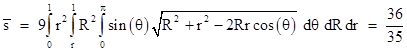
We can restrict our analysis to just the case R > r because the other case (R < r) is symmetrical and has the same distribution of distances.  Hence we need only integrate the distance function with the appropriate weights for the ranges r = [0,1], R = [r,1], and θ = [0,π], and then divide the result by the triple integral of just the weights (rR)² sin(θ), which is 1/9.  This gives the mean distance

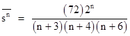
We can also evaluate this integral with the distance function raised to any integral power, to give the average of the nth powers of the distances

Notice that the weight for θ is very fortuitous, because the factor of sin(θ) enables us to evaluate the integral in closed-form, using the easy integral for

In contrast, the seemingly simpler case of a unit disk is actually more difficult because it lacks this convenient weight factor.  It's also worth noting that if we try to cover both the cases R > r and R < r at once by integrating over r = [0,1] and R = [0,1] we are led to a result like 21/20 instead of 36/35.  The subtle problem here is that the integral of

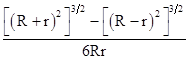
over the range θ = [0,π], divided by the integral of the weight, is

which is formally symmetrical in R and r.  Now, since R+r is always non-negative there's not much ambiguity in evaluating the left hand term in the numerator; we just take the positive value (R+r)³, glossing over the fact that there's really a square root there in the 3/2 power (which means we could have taken the negative root).  However, the right hand term requires a bit of thought: Do we evaluate it as (R–r)³ or (r–R)³ ?  The answer depends on whether R > r or R < r.  In these two cases the above expression reduces to

so it's necessary (not just convenient) to treat the cases separately.  Fortunately, due to symmetry, the cases give the same distribution of distances, so we need only evaluate one of them.

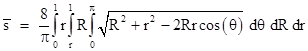
Now let's consider the distances on a unit disk.  This case can be formulated in essentially the same way as with the unit sphere, except that the weights are different.  Each angle θ now represents only a single point, so it's weight is just 1.  Each radius r and R now represents a circle with length proportional to r and R respectively, so these are the weights. The triple integral of the product of these weights is π/8, so the average distance on a unit disk can be expressed as

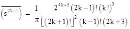
Unfortunately this integral isn't as easy to evaluate as the one for the sphere, because it lacks the sin(θ) factor. We will describe a much simpler approach later, so rather than presenting the elaborate integration here, suffice it to say that the result is 128/(45π). We can also evaluate the above integral for any integer power of the distance function.  For odd powers of the form 2k–1 the general result is

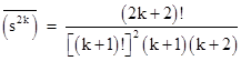
whereas for even powers of the form 2k the general result is

Thus the average squared distance between two point in a unit disk is 1, and the average cubed distance is 2048/(525π). Incidentally, this last formula shows that if C_n denotes the nth Catalan number, then the average (2k)th power of distances on a unit disk is just C_k+1/(k+1).

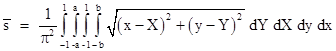
As an alternative to the preceding triple integral, we could just integrate the unit disk by scanning two points (x,y) and (X,Y) orthogonally across the disk.  The weight factors are all 1 in this case, and their product integrates to the squared area of the disk, π², so we have the quadruple integral

where a = (1–x²)^1/2 and b = (1–X²)^1/2.  This gives the same results as the previous triple integral, but it's even more laborious to integrate. We will show later a single integral that gives the same results.

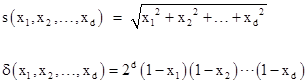
As a way of introducing the simpler method for evaluating the average distances in arbitrary bounded regions, let's first consider the distribution of distances on a 1x1 unit square.  We could use the rectangular approach of the preceding equation and just integrate the distances between two points (x,y) and (X,Y) as each parameter ranges from 0 to 1, but the resulting quadruple integral is not very easy to evaluate.  A much more efficient approach is to notice that the distances and densities (weight factors) on a unit square are distributed according to the parametric formulas

Therefore, we just need to integrate the product δ(u,v) s(u,v) as u and v range from 0 to 1.  The orthogonal way of formulating this double-integral is

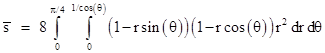
This is a big improvement over the quadruple integral, but it still is not easily evaluated in closed form.  Let's try polar coordinates in this parametric space by setting u = r cos(θ)  and  v = r sin(θ) and integrating over the region u < v  by letting r range from 0 to 1/cos(θ) at each θ from 0 to π/4.  For any incremental slice of θ the weight at r is proportional to r, and of course the integral of r over this region u < v is just 1/2, so we have the integral

The value of this double-integral is

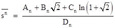
By incrementing the exponent of r in the integral we can evaluate the average of the nth powers of distances on the unit square.  In general the results are of the form

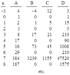
where the values of A, B, C, D are as shown below

The expression doesn’t converge for n = −2 (inverse square), but it does for any real exponent up to that value. The mean of the nth powers reaches a minimum of about 0.114764 for n=9.62, and thereafter increases.

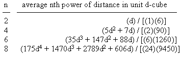
Now, what about the unit cube, or the unit 4D hyper-cube?  The nice thing about the parametric distance density equations is that they immediately generalize to higher dimensions.  The parametric equations for the distance density of a d-dimensional unit cube are

For even powers of the distance we can immediately evaluate the d-dimensional analogs of equation (1).  We find that the average squared distance in a d-dimensional unit cube is simply d/6.  (This gives a nice trivia question: In what dimensional space is the average squared distance in a unit cube equal to unity?) The average nth powers of distances in a d-dimensional unit cube are given by the following formulas for the first few even values of n:

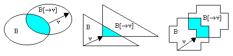
Returning to the parametric density formulas for the distances inside a d-dimensional cube, notice that in each case the density of the vector v = [x₁, x₂, .... x_d]  within a bounded region B is proportional to the intersection of B with a copy of B shifted by the vector v.  More generally, given any finite bounded region B in k-dimensional space, and any k-vector v, let B[→v] denote the image of B translated by v.  Then the density of distances with the magnitude and direction of v is proportional to the content (volume) of the intersection of B with B[→v].  This is because B is the set of possible starting points for the vector v, and B[→v] is the corresponding set of end points.  A particular instance of v (with a particular starting point in B) is a distance between two points of B if and only if its end point is also in B.  Thus, the intersection of B[→v] with B (divided by the content of B itself) is the proportion of points in B for which the vector v is a distance to another point in B.  This is illustrated for a few simple shapes below.

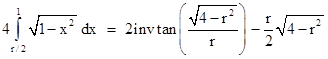
Let's apply this principle to determine the distribution of distances (between two randomly chosen points from a uniform distribution) on a unit disk (radius 1).  For any 2-vector v = [r sin(θ), r cos(θ)] the density is proportional to the overlap of two unit circles with centers a distance r apart.  This is given by

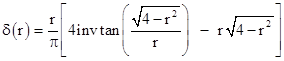
Now, in terms of the parametric lattice of distance vectors (which can be seen as the first quadrant of a circle of radius 2), the number of vectors with magnitude r is proportional to r, so the overall density of distances of magnitude r is proportional to r times the above quantity.  The integral of this resulting function from r = 0 to 2 is simply π/2, so the distribution density of distances on a unit disk is

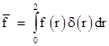
The mean value of any function f of the point-to-point distances is then given by

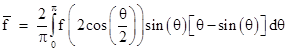
If we make the change of variables r = 2cos(θ/2), the density function can be simplified and we have

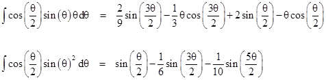
In particular, if f is just the nth power of the distances, we replace the f function with [2cos(θ/2)]ⁿ. Thus for n = 1 we just need the elementary integrals

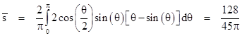
which gives

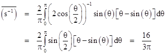
in agreement with the mean distance computed previously by triple and quadruple integrals. An important advantage of this approach is that it not only gives a simpler integration, it gives the entire distribution explicitly, rather than just the mean. Using this same density distribution we can compute the mean value of any function of the distances. For example, the mean of the inverse distances 1/s in a unit disk is given by

(The integral is even simpler in this case.) For a disk of radius r this is simply 16/(3πr). Thus, given n points uniformly distributed on a disk of radius r, there are n(n–1)/2 point-to-point distances, which implies that the expected sum of the inverse distances is 8n(n–1)/(3πr). It’s interesting that while the mean reciprocal distance is finite, the mean squared reciprocal distance is not. This suggests a geometrical version of the Petersburg paradox: the game is to choose two points randomly from a uniform distribution inside a unit circle, and pay an amount proportional to the inverse square of the distance between them. Intuitively it might seem as if the payout would not be very high, but the expected value is actually infinite. (Unlike a sequence of coin tosses, this is a one-step game, but of course we assume infinite precision in the definition of the selected points.)

The proposition that the density of v is proportional to the intersection of B with B[→v] is very general, and applies to non-convex (and even non-connected regions), not just simple regions like spheres and cubes.  For example, it can be used to determine the distance distribution for points of a torus.

Return to MathPages Main Menu