A Four-Component Failure Condition

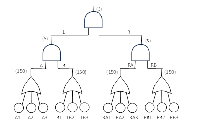
Consider  the fault tree shown below.

Entering this specification into a typical fault tree analysis program would yield 81 cutsets, but by aggregating the sets of three basic inputs to the low-level OR gates, this is really just a single cutset with four inputs, LA, LB, RA, and RB. The numbers in parentheses are the hours for which the condition could latently persist before being checked and repaired.

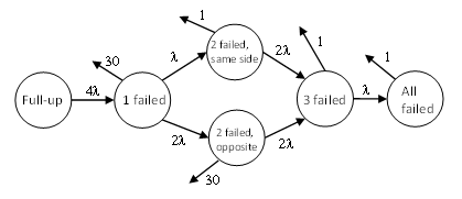
After aggregation, the cutset consists of the joint occurrence of the four conditions. We could apply the general 4-element Markov model, with all 16 possible states, but if each of the four aggregated states has the same probability, λ = λ_LA1 + λ_LA2 + λ_LA3, etc., it’s much more efficient to take advantage of this symmetry to enable the use of a 6-state model shown below.

The backward-going arrows represent the inspection/repair intervals, expressed in terms of the number of 5-hour mission durations. Thus the states with 5-hour exposure are repaired prior to each mission, and the states with 30-hour exposure are repaired every 30 missions. Note that the condition of two failures on the same side (such as LA and LB) is detectable because of loss of function on the left side, whereas two failures on opposite sides is not a detectable condition, because both sides are still functional, so it isn’t checked/repaired until the 30-flight interval.

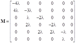
The rate matrix for this system is as shown below.

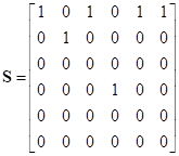
The repair transition matrix, that restores states 3, 5, and 6 back to state 0 after each mission, is

We need only evaluate the probabilities for the first N=30 missions, because after that every component is checked good, so the pattern simply repeats. Beginning with the initial state vector P₀ = [ 1  0  0 0  0  0 ]^T, the probabilities at the ends of the subsequent missions are given recursively by the relation

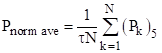
for k=1 to 30, where τ is the mission time (5 hours).  The normalized average probability is then given by

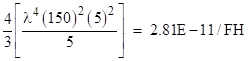
where the subscript “5” denotes the fifth element of the state vector, representing the probability of the top event. For a numerical example, if λ = 1.17E-04/hr, this gives the normalized average probability of 2.70E-11/FH. To show that this is consistent with a more primitive “back of the envelope” calculation, note that the cutset requires two components to fail within a 150-hour period, and two to fail within a 5-hour period, and the number of distinct combinations, counting 1 of 2 from the left and 1 of 2 from the right, is 4, and since there are two “latent” components, the (very) rough averaging factor is 1/(2+1) = 1/3, so we would expect the answer to be somewhere in the neighborhood of

This differs from the exact value of 2.70E-11/FH by only about 4%.

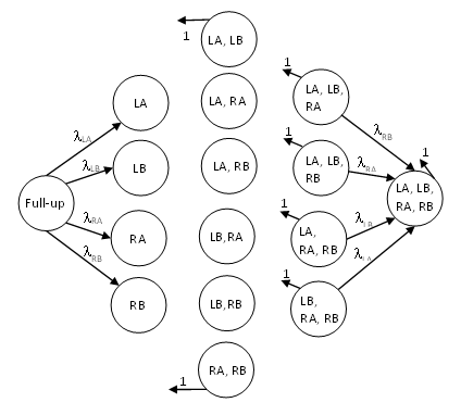
All the above was based on the simplified case where each of the four aggregated basic events has the same failure rate λ. This enabled us to use a simplified model by taking advantage of the symmetry between the four basic events. More generally, if the events LA, LB, RA, RB are allowed to have arbitrary different values, we need to consider the complete four-element model as shown below.

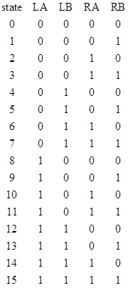
We’ve omitted the transitions to and from the two-fault states (center column), because of their large number, but each transition has the rate associated with the component that is added going from one state to the next. The states with repair intervals of 1 mission are marked, and the remaining failure states are latent with 30 flight inspect/repair intervals. The standard rate matrix for the full n-element model can be generated automatically, as we’ve described elsewhere. For the transition matrix S, we can begin with the 16x16 identity matrix and then move the “1” entries from the diagonal to the top row for the columns corresponding to conditions detectable on one flight. If we use the canonical tiling method to generate the exponential of the rate matrix, the states will be ordered in the binary pattern as shown below.

The states that are detectable and repaired prior to each mission are 3, 7, 11, 12, 13, 14, and 15. With this M and S matrix, we can use the formulas given previously to compute the normalized average probability. In this way we confirm that, setting all of the failure rates to the same value of λ = 1.17E-4/hr, we get (again) 2.70E-11/FH, confirming that the simplified model gives the correct result for the symmetrical case on which it was based.

Return to MathPages Main Menu