Dual Sensor or Channel Failure

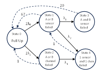
Suppose we have a dual-channel device, and each channel includes a sensor for a certain parameter. Complete loss of that parameter can result from either losing the sensor in both channels, or from having one channel completely inoperative and losing the sensor in the operative channel. (The condition of both channels being inoperative results in a broader loss of function, in which case the loss of the parameter is irrelevant, so this case is not included in the analysis.) Suppose further that the system is checked/repaired for single sensor failures every 500 hours, and that we check for and repair dual sensor failures every 150 hours. (The latter might actually be “on condition”, meaning the clock starts when the condition arises, but it’s satisfactory to treat it as a periodic inspection, since this gives the same maximum persistence time.) An inoperative channel is repaired before each dispatch. Assuming an average flight duration of τ = 7.5 hours, these inspection/repairs are performed every 67, 20, and 1 flight(s), respectively. Letting λ₁ and λ₂ denote the failure rates of sensors and channels respectively, the Markov model for this system is as shown below.

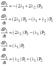
The homogeneous failure equations for the system are

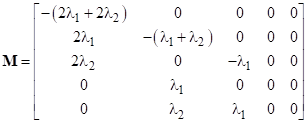
The failure rate transition matrix M for this system is therefore

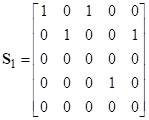
There are three repair transitions to be applied, at intervals of 1, 20, or 67 flights. The first of these is applied before each flight, and it sweeps the probability from State 2 back to State 0, and from State 4 back to State 1. Thus, on each iteration we apply the repair transition matrix

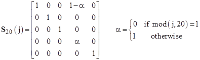
The next repair transition, applied every 20^th flight, sweeps the probability from State 3 back to State 0, so it is defined as

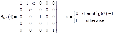
The next repair transition, applied every 67 fights, sweeps the probability from State 1 back to State 0, so it is defined as

We can now compute the probabilities for each of the states on each flight using the recursive relation

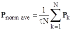
Where τ is the average flight duration and P_k is the probability vector for the kth flight, beginning with the initial condition P₀ = [1 0 0 … 0]^T. The normalized average probabilities for the states are then given by

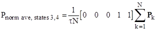
The condition representing the hazard is States 3 and 4, and we can write the normalized average scalar probability for those two states as

To illustrate, suppose we have λ₁ = 6.24E-06/hr and λ₂ = 9.06E-06/hr, and recall that our average flight duration is τ = 7.5 hours. We also stipulate that the life of the airplane is N=14,400 flights. The result is a normalized average probability for the union of states 3 and 4 of 2.33E-07/FH.

Return to MathPages Main Menu