Reliability Calculations with Complex Repairs

The days of our years are threescore years and ten; and if by reason of strength they be fourscore years, yet is their strength labour and sorrow; for it is soon cut off, and we fly away.

                                                                                               Psalm 90:10

In the simplest reliability models the basic components have defined exposure times, representing their inspection/repair intervals, and there are no defined exposure times for the higher-order states of the system. However, in practice, it’s not uncommon to have limited exposure times for combinations of failures that differ from the exposure times for the individual components.

For a very simple example, consider a system consisting of two components, designated as A and B, with constant failure rates λ_A and λ_B, each checked and (if necessary) repaired every 1000 hours, but suppose in addition that an alert is generated if both components are failed, and the system is checked for this alert and (if necessary) repaired back to the full-up state every 200 hours. What is the normalized average probability of the dual-fault condition?

One common way of modeling such a system is by means of a fault tree, but we can’t use a simple AND gate with the two components, each with 1000 hour exposure times, because this wouldn’t account for the 200 hour limitation on the combined state. The usual approach when we have two components with long individual exposure times T_L and a short exposure time T_S for the combined state is to consider the region of the time-time space in which the possible times t_A,t_B of failure for the two components are depicted as shown in the figure below. Here we make use of the rare event approximation, so the probability density is essentially constant over this square region.

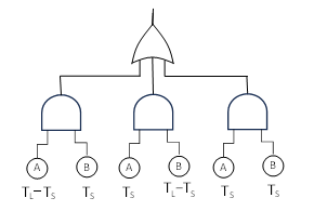
The probability of the dual fault condition being present on the last flight is equal to the probability of the dual-fault condition arising during the last short interval of duration T_S, which can be shown by adding up the probabilities for the flights during that last short interval, after the last dual-fault check/repair that occurs at T_L – T_S. Thus, the probability is proportional to the shaded region in the above figure. These three terms can be represented as branches of a fault tree, with the exposure times as shown below:

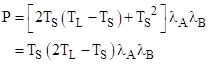
On this basis, the probability of the combined failure condition being present on the last flight is

Since each term involves two components, they increase quadratically with time, so the average can be conservatively approximated by a factor of 1/3 (which is the coefficient of the integral of t²), and the “normalized” value is found by dividing the average probability by the average flight duration T_f, so this gives the approximation of the normalized average probability

To give a numerical example, suppose the failure rates are λ_A = 6E-06/hr and λ_B = 8E-06/hr, the average flight length is T_f = 6 hours, the short interval is T_S = 150 hours, and long interval is T_L = 600 hours. The above formula then gives an approximate value of P = 4.2E-07/FH for the normalized average probability.

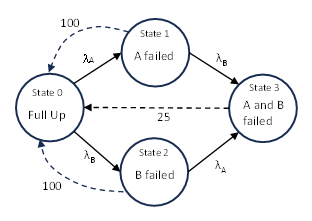
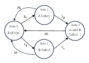
As noted, several approximations were used in arriving at this result. For a more rigorous approach, we can represent the system by a Markov model as shown below.

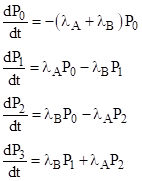
The dashed transitions are sweep resets, performed every 100 or every 25 flights, as marked, with the stipulation that the average flight duration is 6 hours. The homogeneous system equations are

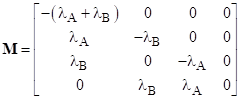
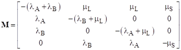
The homogeneous transition matrix M is therefore

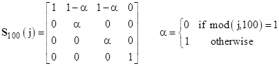
The first periodic sweep matrix, applied every 100^th flight, sweeps the probability from States 1 and 2 back to State 0, so it is defined as

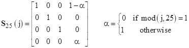
The next periodic sweep matrix, applied every 25 fights, sweeps the probability from State 3 back to State 0, so it is defined as

We can now compute the probabilities for each of the states on each flight using the recursive relation

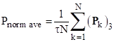
Where τ is the average flight duration and P_k is the probability vector for the kth flight, beginning with the initial condition P₀ = [1 0 0 0]^T. The normalized average probability for State 3 (the dual failure state) is then given by

As an example, using the same parameters given previously, the result is a normalized average probability for States 3 of 3.43E-07/FH. This is roughly 20% lower than the approximate result given by the primitive fault tree calculation.

One might wonder if it is necessary to handle the repair transitions as separate periodic sweep operations. An alternative is to represent those transitions by ordinary Markovian transitions with rates matched to give the same average dwell times. The long and short intervals would be represented by transitions with rates μ_L = 2/600 and μ_S = 2/150 respectively. This is because the fault can occur uniformly (for rare events) in the interval, so the average dwell time is half the interval. The diagram of this fully Markovian model is shown below, with the dashed periodic lines replaced with solid Markovian transitions.

The transition matrix for this model is

We can now compute the probabilities for each of the states on each flight using the recursive relation

Since we have modeled all the repair transitions as Markovian flows, there are no “sweep” operations needed. As before, the normalized average probability for State 3 is given by

Using the same parameters given previously, the result is a normalized average probability for States 3 of 3.56E-07/FH, which is within 4% of the exact result for the strictly periodic repair model.

One could also question whether it is necessary to apply the transient model. The reason for using the transient calculation as the benchmark is that it doesn’t rely on any assumptions about whether the system achieves steady state. If a system contains latent faults that can persist for the life of the airplane, then we can’t be sure the airplane probability will reach steady-state during its life, so we need to use the transient model, which of course also works for systems that reach steady state, and thus has unrestricted validity.

However, in many circumstances, the population of systems clearly reaches steady state, such as for individual engine shutdowns, which occur at a stable rate in the fleet. In contrast, catastrophic failures at the airplane level are many orders of magnitude less probable, so we can’t infer from experience that an airplane has reached a steady-state level. However, even for airplane systems, unlimited exposure times for latent failures are strongly discouraged, so we often have systems with reasonably short exposure times in comparison with the airplane life. This is certainly the case in our numerical example. In such cases, we are assured that the average probabilities reach steady state, so it isn’t necessary (although it is always permissible) to use the transient model.

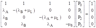
To find the steady-state solution, we need to note that the transition matrix has zero determinant, and hence has no inverse, because the rows identically sum to zero, so they are not independent, i.e., given any three of the rows, the fourth is fully determined. So, to solve for the steady-state solution, we need to replace one of the rows (typically the first, for convenience) with some independent condition, namely the conservation identity

So, we have the steady state equations

Writing these as AP = C, the algebraic solution is simply P = A⁻¹C, which for our numerical example directly gives the normalized result P₃/τ =  3.58E-07/FH. As expected, this is nearly identical to the result given by the transient model.

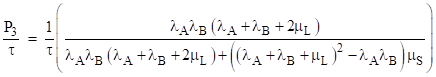
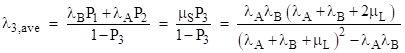
Incidentally, we can write out the steady-state solution for this simple model explicitly as

We can also write down explicitly the steady-state rate of entering State 3 in terms of the steady-state probabilities, which gives

As discussed elsewhere, this is independent of μ_S because the rate of entering State 3 does not depend on how long the system dwells in that state after entering it, whereas the probability of being in State 3 clearly depends on the dwell time, as well as the entry rate. In our numerical example, the steady-state rate is 2.86E-08/hr, which is an order of magnitude lower than the normalized average probability. This is why regulatory safety requirements are expressed in terms of the normalized average probability, not the rate.

Note also that, in the rare event approximation, the value of 1 – P₃ is virtually 1, so we have the approximate relation λ_3ave = (μ_S τ)(P_3ave/τ). This is why the average rate is roughly equal to the normalized average probability multiplied by 2τ/T_S, i.e., the ratio of the average flight length to the average exposure time for the top event. Needless to say, if the top event is latent with a very long exposure time, the average rate can be many orders of magnitude smaller than the normalized average probability. This, again, is why regulatory safety requirements are expressed in terms of the normalized average probability, and it shows clearly why misunderstandings of how latent risk is quantified are equivalent to misunderstandings of normalization.  Even after recognizing that the correct measure of latent risk is the probability of being in the failed state on a given flight, not the probability of entering the failed state on that flight, it’s important to correctly apply normalization by the average flight length, remembering that the purpose of normalization is not to convert a probability to a rate, but simply to re-scale the probability by the average flight length of the particular airplane model, so that the quantitative thresholds correspond to the same number of fatalities per passenger mile on all models. (See Note 2 of this article for the background on the regulatory concept of normalized probabilities.)

Return to MathPages Main Menu