Fractional Calculus

Differentiation and integration are usually regarded as discrete operations, in the sense that we differentiate or integrate a function once, twice, or any whole number of times. However, in some circumstances it’s useful to evaluate a fractional derivative. In a letter to L’Hospital in 1695, Leibniz raised the possibility of generalizing the operation of differentiation to non-integer orders, and L’Hospital asked what would be the result of half-differentiating x. Leibniz replied “It leads to a paradox, from which one day useful consequences will be drawn”. The paradoxical aspects are due to the fact that there are several different ways of generalizing the differentiation operator to non-integer powers, leading to inequivalent results.

In some ways the most natural and appealing generalization is based on the exponential function f(x) = e^ax, whose nth derivative is simply aⁿe^ax. This immediately suggests defining the derivative of order ν (not necessarily an integer) as

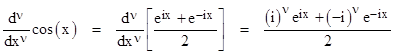
Negative values of ν represent integrations, and we can even extend this to allow complex values of ν. Any function expressible as a sum of exponential functions can then be differentiated in the same way. For example, the generalized derivative of the cosine function according to this approach is given by

Since (±i)^ν = e^±νp/2, we have the nice result

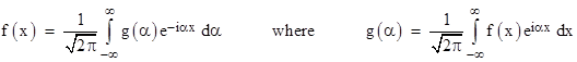
Thus the generalized differential operator simply shifts the phase of the cosine function (and likewise the sine function) in proportion to the order of the differentiation. Needless to say, this approach can be applied to the exponential Fourier representation of an arbitrary function to define the generalized derivative and integral. Recall that the exponential Fourier representation of a function f(x) is defined as

The functions f and g are Fourier transforms of each other. Given the representation of f(x) (meaning that we are given the “coefficient function” g(α)), the generalized derivatives (and integrals) are simply

Hence if g(α) is the Fourier transform of f(x), then the Fourier transform of the generalized νth derivative of f(x) is (-iα)^νg(α).

The exponential approach seems to give a very satisfactory way of defining fractional derivatives… but we have yet to answer L’Hospital’s question, which was to determine the half-derivative of f(x) = x. There is no Fourier representation of this open-ended function, so it has no well-defined spectral decomposition. Of course, we can find the Fourier representation of x over some finite interval, but what interval should we choose? This ambiguity gives a hint of why Leibniz considered the subject to be paradoxical. Leibniz was well aware that the result of integrating a function is neither unique nor local, because it depends on how the function behaves over the range for which the integration is performed, not just at a single point. But he was used to thinking of differentiation as both unique and local, because whole derivatives happen to possess both of those attributes. The apparent paradoxes of fractional derivatives arise from the fact that, in general, differentiation is non-unique and non-local, just as is integration. This shouldn’t be surprising, since the generalization essentially unifies integrals and derivatives into a single operator. If anything, we ought to be surprised at how this operator takes on uniqueness and locality for positive integer arguments.

To get a clearer idea of the ambiguity in the concept of a generalized derivative, it’s useful to examine a few other approaches, and compare them with the exponential approach described above. The most fundamental approach may be to begin with the basic definition of the whole derivative of a function f(x)

Repeated composition of this operation leads to

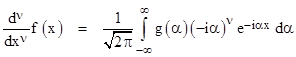
for any positive integer n. To illustrate, this formula gives the second derivative of the function f(x) = x⁴ as

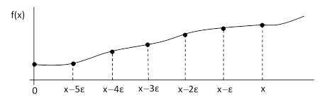
We can generalize equation (1) for non-integer orders, but to do this we must not only generalize the binomial coefficients, we also need to determine the appropriate generalization of the upper summation limit, which we wrote as n in equation (1). To clarify the situation, let us go back and derive “from stratch” the operations of differentiation and integration in a unified context. Consider an arbitrary smooth function f(x) as shown in the figure below.

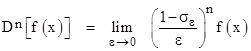
In addition to the point at x, we’ve also marked six other equally-spaced values on the interval from 0 to x, each a distance ε from its neighbors. The number k of these points is related to the values of x and ε by x = kε. For convenience, we define a shift operator σ_ε such that σ_εf(x) = f(x-ε). Now we consider a general operation D defined by

Recalling the geometric series expansion 1/(1-z) = 1 + z + z² + z³ + …, the effects of this operator with n = +1 or -1 are

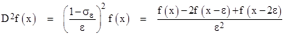
in the limit as ε goes to zero. Thus we see that D is simply the differentiation operator, and its inverse, D^-1, is the integration operator. This reproduces the ordinary whole derivatives. For example, the second derivative of f(x) is

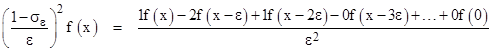
in the limit as ε goes to zero, which illustrated how we recover the binomial equation (1) for any whole number of differentiations. However, strictly speaking, this context makes it clear that we should actually write the second derivative as

It just so happens that, if n is a positive integer, all the binomial coefficients after the first n+1 are identically zero (i.e., we have C(n;j) = 0 for all j greater than n), so we can truncate the series, but for any negative or fractional positive values of n, the binomial coefficients are non-terminating, so we must include the entire summation over the specified range. Consequently, the upper summation limit in (1) should actually be (x-x₀)/ε, where x₀ is the lower bound on the range of evaluation. We often choose x₀ = 0 by convention, but it is actually arbitrary, and we will see below some circumstances in which the lower bound is not zero. In any case, we can re-write equation (1) in the more correct form that does not rely on n being a positive integer

To define the binomial coefficient for non-integer values of n, recall that for integer arguments these coefficients are defined as

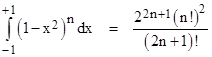
so we need a way of evaluating the factorial function for non-integer arguments. Notice that for any positive integer n we have the definite integral

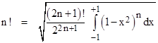
Solving for n! gives

The argument of the factorial on the right side is 2n+1, so the right hand expression is well-defined for half-integer value of n such that 2n+1 is non-negative. Hence this is a well-defined expression for the factorial of any such half-integer argument. For example, setting n = -1/2, we get

Furthermore, now that the factorial of all (positive) half-integers is defined, the above formula allows us to compute the factorial of any quarter-integer, and then every sixteenth, and so on. Hence, using the binary representation of real numbers, and using the identity (x+1)! = (x+1)x!, we now have a well-defined factorial function for any real number. This is traditionally called the gamma function, with the argument offset by 1 relative to the factorial notation, so we have

for any positive integer n. The fundamental recurrence formula for the gamma function is therefore Γ(x+1) = x Γ(x). Thus we have the following values for positive half-integer arguments

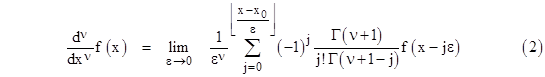
Note the reflection relation Γ(x) Γ(1 – x) = π / sin(πx). Now that we have a general way of expressing “factorials” for non-integers, we can re-write equation (1a) in generalized form, replacing each appearance of the integer n with the real number ν. This gives

If ν is an integer n, the vanishing of the binomial coefficients for all j greater than n implies that we don’t really need to carry the summation beyond j = n, and in the limit as ε goes to zero the n values of f(x-kε) with non-zero coefficients all converge on x, so the derivative is local. However, in general, the binomial expansion has infinitely many non-zero coefficients, so the result depends on the values of x all the way down to x₀. We typically choose x₀ = 0, so we are effectively evaluating the “derivative” (which is not the same as the “slope”) for the interval from 0 to x. Thus, as mentioned previously, the generalized derivative is a non-local operation, just as is integration. The general derivative depends on the value of the function f over the whole range from x₀ to x. This can be seen from the factor f(x – jε) in the summation in equation (2), showing that as j ranges from zero to (x – x₀)/ε the argument of f ranges from x down to zero. It just so happens that this non-locality disappears for positive whole derivatives. (This simple mathematical fact has an important consequence in the strong form of Huygens’ Principle, which accounts for the sharp propagation of light and other wavelike phenomena in three dimensional space.)

Choosing x₀ = 0 as the low end of our differentiation interval, the formula (2) for the general derivative becomes

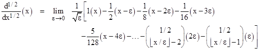
With this, we are finally equipped to attempt to answer L’Hospital’s question. Taking the function f(x) = x with ν = 1/2, signifying the half-derivative, this formula gives

In this equation the binomial coefficients symbol is understood to denote the generalized function, with the factorials expressed in terms of the gamma function. As explained previously, the coefficients in the above expression are just the coefficients in the binomial expansion of (1 – σ_ε)^1/2.  Evaluating this expression in the limit as ε goes to zero, we find that the half-derivative of x is

This is exactly what we would expect based on a straightforward interpolation of the derivatives of a power of x. Recall that the first few (whole) derivatives of  x^m  are

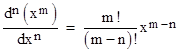
Thus we expect to find that the general form of the nth derivative of x^m is

Replacing the integer n with the general value ν, and using the gamma function to express the factorial, this suggests that the a fractional derivative of xⁿ is simply

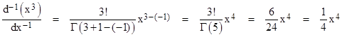
which is exactly the same answer to L’Hospital’s question as we got previously, i.e., the half-derivative of x is given by (4). Now, since analytic functions can be expanded into power series, we can use equation (5) to determine the fractional derivatives of all such functions. Furthermore, applying this formula with negative values of ν gives a plausible expression for the integral of a power of x. For example, to find the whole integral of x³ we set m = 3 and ν = –1, and then compute

So, in a sense, equation (5) is an algebraic expression of the fundamental theorem of calculus, i.e., the inverse relationship between the operations of differentiation and integration, since the nth derivative of the –nth derivative (integration) is the identity. The unification of these two operations makes it even less surprising that generalized differentiation is non-local, just as is integration.

Incidentally, the generalized derivative as developed so far gives some slightly surprising results. For example, the half-derivative of any constant function cx⁰ is

Thus, not only is the half-derivative of a constant with (respect to x) non-zero, it is infinite at x = 0. Nevertheless, equations (3) and (5) are agreeably consistent with each other, giving some confidence in the significance of this generalization of the derivative. Given this equivalence, one might wonder about the value of the elaborate derivation of equation (3) when it seems to be so much easier and more direct to arrive at equation (5). In answer to this there are two points to consider. First, equation (3) applies to fairly arbitrary functions, whereas equation (5) applies only to functions expressible as power series. Still, a very large class of functions can be expressed as power series, so this in itself is not an overriding factor. More important is the fact that equation (5) gives no hint of the non-locality of the generalized derivative, i.e., the dependence on the function over a finite range rather than just at a single point, and the need to specify (implicitly or explicitly) the chosen range. The importance of this can be seen in several different ways. Perhaps the most significant reason for taking care of the derivative interval is brought to light when we try to apply equation (3) or (5) to the simple exponential function. We previously proposed that the general nth derivative of e^ax is simply (a)ⁿ e^ax, and yet if we expand the exponential function e^x into a power series

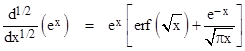
and apply equation (5) to determine the half-derivative, term by term, we get

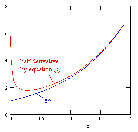
A plot of this function, along with e^x, is shown in the figure below

Here we see one of the paradoxes that might have intrigued Leibniz. According to a very reasonable general definition we expect any derivative (including fractional derivatives) of the exponential function to equal itself, and the exponential goes to 1 as x goes to zero, and yet our carefully-derived formulas for the half-derivative of the exponential function goes to infinity at x = 0. Clearly something is wrong. Must we abandon the elegant exponential approach, along with it’s beautiful explanation of the trigonometric derivatives as simple phase shifts, etc? No, we can reconcile our results, provided we recognize that the derivative is non-local, and therefore depends on the chosen range of differentiation. Consider the two anti-differentiations shown below

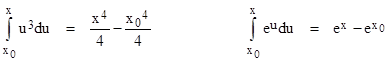
The left-hand integral shows that when we say x³ is the derivative of x⁴/4 we are implicitly assuming x₀ = 0, which is consistent with our derivation of equation (3). However, the right-hand integral shows that, by saying e^x is the derivative of e^x, we are implicitly assuming x₀ = –∞. Thus ranges of integration/differentiation we have tacitly assumed for these two definitions are different. To get agreement between the interpolated binomial expansion method and the definition based on exponential functions we must return to equation (2), and replace the condition x₀ = 0 with the condition x₀ = –∞. This is easy to do, because it simply amounts to setting the upper summation limit to infinity, i.e., we take the following formula for our generalized derivative

With this, we do indeed find that the νth derivative of e^ax is simply (a)^νe^ax, consistent with the purely exponential approach.

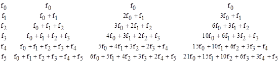
Still another approach to fractional calculus is to begin with a generalization of the formula for repeated integration. Suppose the function f(x) has the specified values f₀, f₁, f₂, f₃, f₄, and f₅ at equally spaced intervals of width ε. The integral of this function from x = 0 to 5ε can be approximated by ε times the cumulative sum of these values, and the integral of this new function is ε times the cumulative sum of those values, and so on. This is illustrated in the table below.

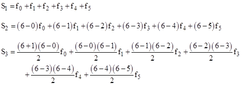
Thus the 1st, 2nd, and 3rd “integrations” yield the values

As we divide the overall interval into more and more segments, ε becomes arbitrarily small, and so do the differences between the factors in any given term, so the successive integrations give

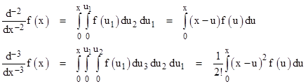
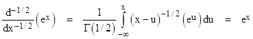
and so on. Thus we have Cauchy’s expression for repeated integrals, which we can express using the gamma function instead of factorials, as

The convergence properties of this formula are best when ν has a value between 0 and 1. There are two different ways in which this formula might be applied. For example, if we wish to find the (7/3)rd derivative of a function, we could begin by differentiating the function three whole times, and then apply the above formula with ν = 2/3 to “deduct” two thirds of a differentiation, or alternatively we could begin by applying the above formula with ν = 2/3 and then differentiate the resulting function three whole times. These two alternatives are called the Right Hand and the Left Hand Definitions respectively. Although these two definitions give the same result in many circumstances, they are not entirely equivalent, because (for example) the half-derivative of a constant is zero by the Right Hand Definition, whereas the Left Hand Definition gives for the half-derivative of a constant the result given previously as equation (6). In general, the Left Hand Definition is more uniformly consistent with the previous methods, but the Right Hand Definition has also found some applications.

Equation (8) highlights (again) the non-local character of fractional operations, because it explicitly involves an integral, which we have stipulated to range from 0 to x. For any whole number of differentiations we don’t need to invoke this integral, but for a non-integer number of differentiations we must include the effect of this integral, which implies that the result depends not just on the values of f at x, but over the stipulated range from 0 to x.

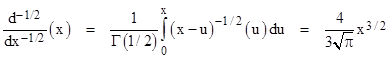
To illustrate the use of equation (8), we will (again) determine the half-derivative of f(x) = x, as L’Hospital requested. Using the Left Hand Definition, we first apply half of an integration to this function using equation (8) with ν = 1/2, giving

Then we apply one whole differentiation to give the net result of a half-derivative

in agreement with equation (6). In this case the Right Hand Definition gives the same result.

Now suppose we apply this method to the exponential function. Since our definition has been based on the range from 0 to x, whereas we’ve seen that the “exponential approach” to fractional derivatives is essentially based on the range from –∞ to x, we expect to find disagreement, and indeed for the half-derivative of e^x we get (by applying (8) with ν = 1/2 and then differentiating one whole time)

This is identical to the half-derivative of e^x given by equation (5), shown in red in the plot presented previously (when we only had the series expansion of this function). Again, we can reconcile this approach with the “exponential approach” by changing the lower limit on the integration from 0 to –∞. When we make this change, equation (8) gives

and of course the whole derivative of this is also e^x, so the half-derivative of e^x by this method is indeed e^x, provided we use a suitable range of differentiation.

Return to MathPages Main Menu