Probability for Regulatory Requirements

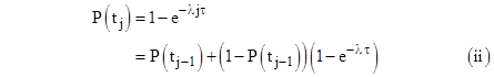
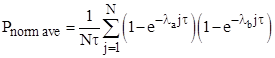
Regulatory requirements state that the numerical probability thresholds for various hazard levels apply to a quantity called “Average Probability per Flight Hour”, also known as the normalized average probability. This quantity is defined as the average of the probabilities of a given failure condition on the flights in the life of the airplane (or the least common multiple of the detection/repair intervals), divided by the average flight length, τ, of the model. For an element with constant failure rate λ (no phase dependence) that is checked and (if necessary) repaired before each flight, the probability of being failed at the end of the jth flight is

Thus, for this simple example, the probability of the failure condition at the end of each flight is the same. On the other hand, if failures of the element are latent (never checked or repaired) for the N flights in the life of the airplane, meaning a latency period of T = Nτ, the AC says the probability of being failed at the end of the jth flight is

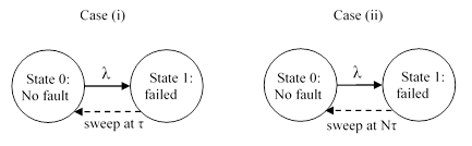
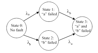
for j = 1 to N. These two cases (i.e., detected/repaired at an interval τ or an interval Nτ) can be represented by the simple Markov models shown below.

As an aside, we note that if the model were embedded in a larger model, there might be a transition from State 1 to (say) a high-level catastrophic failure event, but typically such a transition rate would be less than 1E-05/hr (limiting the so-called “residual” probability), which corresponds to a repair transition of about 100,000 hours, i.e., greater than the life of the airplane, so such a transition typically has no significant effect on these states.

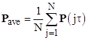
In either of the two cases (i) and (ii), the average of the per-flight probabilities of State 1 (meaning the probability of being in state 1 at the end of the jth flight) is given by

where K is the number of flights between inspections/repairs. In the case where the failure is obvious and is detected and (if necessary) repaired before each flight, we have K = 1, whereas in the other extreme if the system is never checked during the N flights in the life of the airplane, we have K = N. This applies to a cutset with just a single component.

For sufficiently small probabilities we have P(t_j) ≈ λτ for Case (i), and the average of these probabilities for any number of flights is P_ave = λτ, so dividing this by the average flight length τ gives the normalized average probability P_{ave per fh} = λ. On the other hand, for Case (ii) we have P(t_j) ≈ λjτ, and the average for j = 1 to N flights is P_ave = λτN(N+1)/(2N), so for large N the normalized average probability is P_{ave per fh} = (1/2)λT/τ.

For a cutset with n components with constant failure rates λ₁, λ₂, …, λ_n and completely independent inspection/repair intervals K₁, K₂, …, K_n flights, the normalized average probability is given simply by

where N is the least common multiple of the K_i values. (We can also set N to the number of flights in the life of an airplane.) However, if the inspection/repair intervals for the components are not independent, this simple formula can’t be used. For example, we may have two components that are individually completely latent, so each could be failed for the life of the airplane, but if they are both failed, this condition may be detectable and repaired before the next flight. For such a system, equation (2) is not applicable, and we must account for the repair transitions that are applied to combined states.

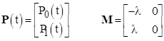
To develop the formula applicable to arbitrary discrete repairs, whether they are for individual failure states or combined failure states, it’s useful to begin by re-deriving the simple case of a single component in matrix form. In terms of the state vector and transition matrix

the homogeneous differential state equations for the Markov model can be written as

Beginning with P(0) = transpose[1  0], the probabilities of the states at the end of the jth flight can be expressed recursively in terms of the probabilities at the end of the previous flight by

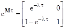
for j = 1 to N, where

which in this simple one-component example is

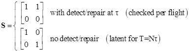
and the detect/repair matrix S is given by

With these S matrices, and noting that P₀(t) = 1 − P₁(t), equation (4) is equivalent to (i) and (ii) respectively. In these terms the averages of each of the states in the model are given by

Making use of the row vector R = [0  1] to select the probability of the “top” event, and dividing by the average flight length τ, we can write the normalized average probability of the failed state (State 1 in this model) in closed form as

The same calculations can be applied to any combination of elements, with any specified detection/repair intervals. For example, given two independent components with constant failure rates λ_a and λ_b, both functional at time t=0, the homogeneous Markov model is shown below.

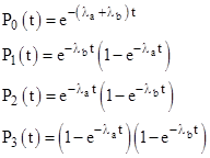
The explicit time-dependent solution of the homogeneous state equations for this two-component system is

Letting τ denote the duration of each flight (all assumed to be of average duration), the normalized average probability of the fully latent failure condition P₃ (both components failed undetected) at the end of the jth flight for the N flights in the life of the airplane is

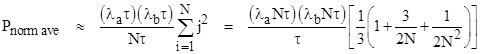
For sufficiently small probabilities (e.g., smaller than 0.01), the expression for P₃(jτ) is closely approximated by P₃(jτ) ≈ (λ_ajτ)(λ_bjτ), so the expression for the normalized average probability is approximately

For large N the factor in square brackets is essentially just 1/3, which is the averaging factor for a combination of two elements with the same latency period. Thus, letting T = Nτ denote the total latency period, we have the familiar approximation P_{ave per fh} ≈ (1/3)(λ_aT)(λ_bT)/τ.

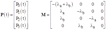
However, if the inspection/repair intervals are not independent, such as if the combination of the two failures would be detected and repaired before the next flight, we need to apply the more general approach that can be expressed using the matrix formalism. In terms of the state vector and transition matrix

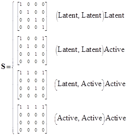
the state equations for the Markov model are given by equation (3), and the state probabilities at the end of the jth flight are given recursively by equation (4). In this case we can have different possible detect/repair matrices S, depending on the detectability and repair transitions, as summarized below:

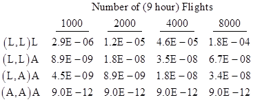
The notation (Latent, Latent)Latent signifies that the two components are individually latent, and they are also latent in combination, and the notation (Latent, Latent)Active signifies that the two components are individually latent but if they are both present they are detected and repaired (or replaced) before the next flight. In these terms, and making use of the row vector R = [0 0 0 0 1], we can compute the normalized average probability for the top state in the model using equation (5).

To illustrate, for a two-component system with λ_a = 1E-06, λ_b = 1E-06, and an average flight length of τ = 9 hours, we get the results tabulated below for latency periods ranging from 1000 to 8000 flights (9000 to 72000 hours).

The above examples apply when each component is either detected/repaired before each flight, or is not detected/repaired for the full N flights in the life of the airplane. More generally, if some detections and repairs occur per flight, and other occur at an interval of N_a flights, and other occur at an interval of N_b flights, the probability at the end of the kth flight is given recursively by

for j = 1 to N, and hence the normalized average probability over the total airplane life of N flights is given by

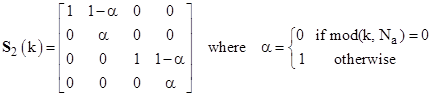
where S₁ is a repair transition applied before each flight, and S₂(j) and S₃(j) are repair transition matrices when j is a multiple of N_a and N_b respectively, and otherwise they are the identity matrix. For example, given the two-component system described above, the repair matrix for component “a” would be

Equation (7) gives the normalized average probability for any combination of any number of components, with any specified detection/repair intervals, consistent with the definition of this quantity in the draft AC 25.1309.

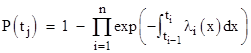
In the preceding discussion we stipulated constant failure rates, consistent with the fact that the AC says “failure rates utilized in calculating the "Average Probability per Flight Hour" should be estimates of the mature constant failure rate”. This means the failure rates are taken to be the same for each flight. However, the failure rates may vary systematically during the course of an average flight, either because of phase dependence (e.g., some failures can only occur during landing) or because of external factors (e.g., the difference in Single Event Upset rates at low versus high altitude). The AC includes provisions to account for this by writing equation (i) in the form

where n is the number of phases, λ_i(x) is the failure rate function for the ith phase, and t_i-1 and t_i denote the beginning and ending times of the respective phases. Now, the product of exponentials of the integrals covering the total flight time from 0 to τ is simply the exponential of the sum of those integrals, so the equation can be written equivalently as

The quantity in square brackets is the mean failure rate during the flight, so we see that our original equation (i) still applies, with the understanding the λ represents the mean failure rate during each flight. The same applies to the failure rate matrix M, i.e., the formulas given previously are still exactly valid with failures rates that vary during the flight, with the understanding the M denotes the mean failure rate matrix.

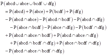
The above discussion gives the probabilities for individual minimal cutsets consisting of the intersection of one or more basic elements. In general an overall failure condition may consist of the union of several minimal cutsets. The probability of the union of cutsets can be computed by applying the usual inclusion/exclusion formula. For example, if abcd, abce, bcdf, and dfg are four cutsets involving the independent elements a,b,…g, we have

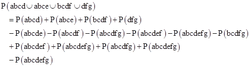
Evaluating the intersections, we get

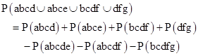
Cancelling terms, this reduces to

Note that the full expression for the probability of the union of n cutsets has 2ⁿ – 1 terms, so (for example) the expression for the combined probability of 30 cutsets has over a billion terms, each of which consists of the probability of the intersection of a subset of those minimal cutsets, which results in non-minimal cutsets that need to be evaluated.  Fortunately the simple sum of the probabilities of the n minimal cutsets is an upper bound on the actual probability of the union, so this is often used as a conservative approximation. For a slightly less conservative approximation (for monotonic mincuts), we can cumulatively apply the second-order recurrence

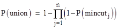
beginning with P(union)₀ = 0. To prove that this is an upper bound, recall that for any two events A, B we have the exact relation P(A U B) = P(A) + P(B) – P(A ∩ B), and for monotonic events, i.e., events constructed using only AND and OR gates, with no negations, we have the relation P(A)P(B) ≤ P(A ∩ B), so the expression P(A) + P(B) – P(A)P(B) is greater than or equal to P(A U B). Hence, applying this recursively by the formula above gives an upper bound on the overall union. As an aside, the upper-bound relation P(A U B) = P(A) + P(B) – P(A)P(B) can also be written in the equivalent form 1 − P(A U B) = [1 − P(A)][1 − P(B)], so the upper bound for the overall union of all the cutsets can be written formally as

This expression is formally succinct, but may not be optimum for calculation, because for cutsets with extremely small probabilities the factors differ from 1 by only very small amounts, so numerically some significant digits may be lost. For this reason, it may be preferable to use the recurrence formula. We also note that, if there is a set of basic events that appears in every cutset, these can obviously be factored out of the entire Boolean expression for the union, and these factors are then independent of the remaining expression, so they can be applied separately. For example, the list of cutsets abcd + abef + abdf can be factored as ab(cd+ef+df), so the probability of the union is P(a)P(b)P(cd+ef+df).

Incidentally, dividing the average per-flight probability by the average flight length (sometimes called “normalization”, although that is a misnomer) was intended to enable a single numerical threshold, such as 1E-09 for catastrophic failures, to be applied to all airplane models, for both long-range and short-range aircraft. The quantity to be regulated is fatalities per passenger mile.  Let k denote the number of passengers per plane, V the average speed of the plane (miles per hour), τ the average hours per flight, and c the expected number of catastrophic flights per flight. The number of passenger miles per hour is kV, and the number of fatalities per hour is kc/τ, so the number of fatalities per passenger mile is (kc)/(kVτ) = (c/V)/τ. Large commercial transport aircraft all typically cruise at roughly the same average speed V ≈ 500 mph, but the average flight length, τ can differ significantly: Short range aircraft may have an average flight length of 1 hour, whereas long range aircraft may have an average flight length of 10 hours. The quantity c/τ is roughly proportional to fatalities per passenger mile for all models.

Occasionally one sees the claim that if the per-flight probability is not uniformly distributed during the flight – such as being concentrated during the takeoff or landing phase, this normalization does not apply, but this claim is contradicted by the fact that the advisory material specifically includes provisions for different failure rates in different phases, as described in another article.

Return to MathPages Main Menu