Latencies and Periodic Repairs

As discussed in another note, the state probabilities for the missions of a system with monotonic failure transition matrix M and average mission time τ, with no inspections/repairs, are given recursively by

for j = 1 to N, where N is the number of missions in the life of the vehicle and P(0) = transpose[1,0,0,…,0]. The normalized average probability is then given by

where R = [0,0,…,0,1].  On the other hand, if there are maintenance actions performed at an interval of N₁ missions, these are applied to equation (1) as follows

where S₁(j) is a matrix that defines the repair transitions when j is a multiple of N₁, and otherwise is the identity matrix.

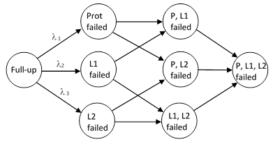
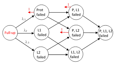
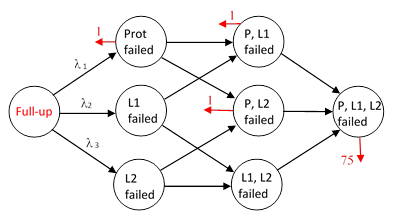
To illustrate, consider a system with a protection feature designed to safely accommodate a certain failure mode, and suppose that protection feature is automatically tested prior to every mission, and if it is found inoperative it will illuminate two different alert lights. To ensure that the protection feature is operational on every mission, it is required to be repaired before the next mission if either of the alert lights is illuminated. However, the alert lights themselves can fail latently. As a result, it is possible for both alert lights to fail, and then the protection system to fail, and this would be a totally latent condition, which could be present for many missions indefinitely. In this condition, if the active failure mode occurs, it would be unaccommodated, resulting in a catastrophic failure.

A generic Markov model of the system consisting of the three potentially latent components (the two lights and the protection feature) with no repair transitions is shown below.

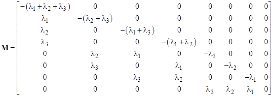
The failure transition matrix is

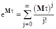
Naturally the exponential of Mτ can be written as the series

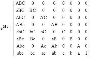
which generally converges rapidly, but we can also express this matrix explicitly in closed form as

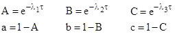
where

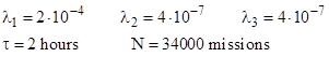
The order of the states in the state vector goes from the full-up state ABC to the state abc with all three components failed. As a numerical example, if we have

equation (2) gives the result P_{norm ave} = 1.205E-04 /FH. However, the states aBC, abC, and aBc each involve the protection function being failed while at least one alert light is working, so these will be detected and repaired before every mission. These per-mission repair transitions are marked on the schematic below.

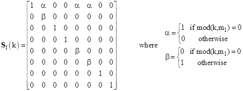
To impose these discrete detect/repairs transitions before each departure, we apply the sweep matrix shown below.

Since we want to repair any probability that has accumulated in those three states back to the ABC state before every mission (which implies that if both lights didn’t illuminate, we would also fix the one that didn’t), we set the interval to m₁ = 1 mission. The probabilities for each mission are then given by equation (3), and then (2) gives the normalized average probability P_{norm ave} = 1.998E-05 /FH.

As an aside, suppose we perform a direct test of the protection function, by external means, before each mission, and repair everything if it is found to be failed. In that case we would place a and b in the upper and lower right corners of S₁ respectively, and equation (2) would give the result P_{norm ave} = 1.357E-09 /FH. Of course, this would be applicable only if we actually had a check and repair before each mission.

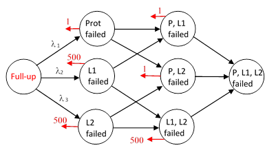
More realistically, we might perform an external check of the protection feature at an internal of, say, 150 hours, which would be 75 missions, as marked in the schematic below.

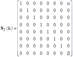
To evaluate this, while still accounting for the normal detection/repair prior to each mission ensured by the alert lights when they are functional, we would use the original S₁ shown above, and apply another sweeping transition S₂ with m₂ = 75 missions. This sweep matrix would move any accumulated probability in state abc back to state ABC, as shown below:

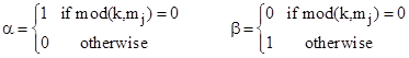
where for each such matrix S_j the parameters a and b are defined by

Applying both S₁ and S₂, the basic recursive formula for the probabilities at the end of each mission becomes

and for the current example equation (2) gives the result P_{norm ave} = 5.153E-08 /FH. This assumes that if the protection is found failed, we troubleshoot and repair the alert lights as well. A slight variation on this strategy would be to apply the external check of the protection feature at 75 missions, but if the protection is found failed, we only repair the protection itself, and do not troubleshoot or fix the alert lights. To evaluate this we would modify S₂ so that instead of sweeping the probability in state abc back to state ABC, we would sweep it back to Abc (i.e., the state in which the protection is working but the lights are still failed). With this modified S₂, equations (4) and (2) give Pnorm ave = 3.511E-07 /FH, so this is a substantially less robust strategy.

A different inspect/repair strategy would be to dispense with the external check of the protection function on every 75^th mission, and instead perform a check of the alert lights every m₃ = 500 missions, as shown in the schematic below.

This is accomplished by the sweep matrix

We don’t need to sweep states aBC, aBc, or abC with this transition, because those are already detected and swept by S₁ on every mission. The recursive formula for this case is

and equation (2) gives the result P_{norm ave} = 1.241E-09 /FH. This shows that checking the light circuits every 1000 hours is significantly more effective than checking the protection function every 150 hours. It’s also worth noting that the results are sensitive to the failure rate of the protection function, perhaps in an unintuitive way. The plot below shows the normalized probability for the 75mission function check and the 500 mission alert check. Since the failure rate of the function may vary, and some units may have much longer MTBF than others, it is something considered prudent to use the value that gives the worst top level probability.

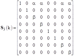
To combine the two maintenance strategies, by checking the alert lights every 500 missions and checking the protection function every 75 missions, we apply both S₂ and S₃ (as well as S₁ for the normal detection on each mission), using the recursive formula

Applying equation (2) then gives the result P_{norm ave} = 3.213E-10 /FH. Thus apply the 75 mission check of the protection feature to the 500 mission check of the alert lights reduces the normalized average probability of the totally latently failed state only by a factor of about 3.

Incidentally, we can also easily compute the failure rate for entering the fully-failed event, which is given at any time by

The average of the values of this rate at the end of each flight is given by

where r = [0, 0, 0, 0, λ₃, λ₂, λ₁, 0]. It’s worth noting that, at least in the small number approximation (i.e., probabilities many orders of magnitude smaller than 1), this is the same as the normalized average probability given by equation (2) for a system with a per-flight inspection/repair on the fully-failed event. As a result, this rate is independent of any actual inspection/repair that we might impose on the fully-failed event, so, for a fully latent condition, equation (7) does not provide a suitable quantification of the risk associated with the latency of that failure condition. In contrast, the normalized average probability given by equation (2) provides an accurate quantification of the risk, with or without latency, so it is generally the appropriate measure. Of course, if the fully-failed event is not latent, as is typically the case for hazardous or catastrophic failure conditions, the two quantities are essentially equivalent. The difference is significant only for totally latent failure conditions.

Return to MathPages Main Menu