|
The Mean Rate Matrix and Diagonalization |
|
|
|
We’re not expecting any surprises, but we won’t be surprised if we find any. |
|
Flight Test Director |
|
|
|
For a single element the failure rate matrix for the homogeneous system is |
|
|
|
|
|
|
|
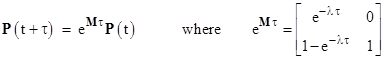
and for any initial state vector P(0) the solution of the system dP(t)/dt = MP(t) is |
|
|
|
|
|
|
|
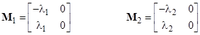
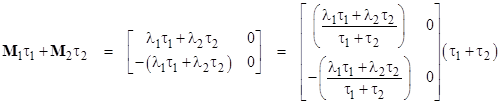
Now suppose we split the time interval τ into two segments, so τ = τ1 + τ2, during which the failure rate has the constant values λ1 and λ2 respectively. The two rate matrices are |
|
|
|
|
|
|
|
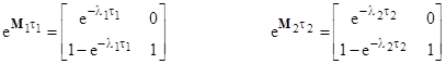
and we have |
|
|
|
|
|
|
|
where |
|
|
|
|
|
|
|
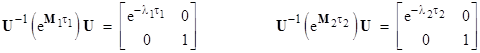
Multiplication of arbitrary matrices is not generally commutative, but a sufficient condition for commutivity is that the matrices are diagonalizable on the same basis. In other words, the multiplication of two matrices A and B is commutative if there exists a matrix U such that U−1AU and U−1BU are both diagonal. It’s easy to show that with the matrix |
|
|
|
|
|
|
|
we have |
|
|
|
|
|
|
|
Therefore multiplication of any two exponential matrices of this particular form is unique, and satisfies the law of exponents, so equation (1) can be written as |
|
|
|
|
|
|
|
This shows that the probability at the end of the two segments is the same, regardless of the order of the segments. Since we have |
|
|
|
|
|
|
|
we can write equation (2) as |
|
|
|
|
|
|
|
where Mmean is the matrix whose elements are the means of the corresponding elements of the individual rate matrices. By the same method we can split up any time span into any number of segments with their individual rates, and the net effect on the state vector is given by this simple formula in terms of the mean rate matrix and the total elapsed time. |
|
|
|
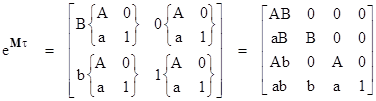
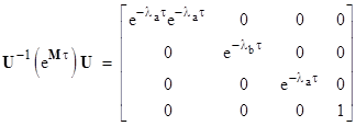
Likewise this applies to the homogeneous solution for any number of components. For example, as described in the article on the tiling product, the exponential of the rate matrix for a system with two components with failure rates λa and λb is |
|
|
|
|
|
|
|
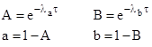
where |
|
|
|
|
|
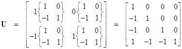
Any matrix of this form is diagonalized by conjugation with the matrix |
|
|
|
|
|
|
|
This is produced by the same tiling operation that yields the exponential of the rate matrix. Forming the conjugate gives the diagonalized matrix |
|
|
|
|
|
|
|
The product of two such diagonal matrices, for two time segments with different rates, consists of a diagonal matrix whose elements are simply the scalar products of the corresponding elements of the two matrices, and the result can be expressed as a matrix of this same form where τ is the combined time interval and the component failure rates are the time-weighted means of the rates over that interval. This confirms that the commutative product of the original exponential matrices is uniquely given by |
|
|
|
|
|
|
|
Consequently the solution for any number of phases can be written in terms of a single exponential using the mean failure rate function and the total time. It should be emphasized that this applies only for the pure monotonic homogeneous form of the system equations, not to arbitrary transition matrices with repairs, i.e., reverse transitions. That is because two such matrices cannot, in general, be diagonalized on a single basis. This is why we can apply this aggregation of segments only over the phases of a single flight when there are potential repairs between flights. Those repair transitions are handled by the application of the “S” matrices in the recurrence formula Pj = eMτ Sj−1 Pj−1. By stipulation, each flight consists of the same set of phase segments with the same failure rates for the individual components, so the same exponential factor using the mean failure rate matrix and flight time can be used in the recurrence. |
|
|
|
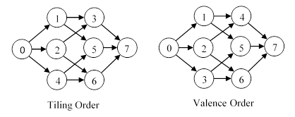
When proceeding to systems with three or more components, there is more freedom in the choice of the ordering of the state equations and the elements of the state vector. Care must be taken to match the numbering of the states and ordering in the state vector to with the tiling pattern. The schematic on the left below shows the ordering that results from the tiling arrangement, whereas the valence ordering on the right proceeds through the first, second, and third order terms in sequence. The difference just amounts to swapping the state equations for states 3 and 4. |
|
|
|
|
|
|
|
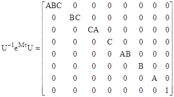
Using the tiling order, the diagonalized rate matrix has the form |
|
|
|
|
|
where |
|
|
|
|
|
|
|
With the valence ordering the middle two rows and columns would be swapped. |
|
|
|
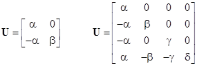
Incidentally, the U matrices described above are not unique, because there are more general matrices that diagonalize these rate matrices. For example, for one or two components we could use the diagonalizing matrices |
|
|
|
|
|
|
|
for any non-zero constants α, β, γ, δ. It suffices to set these constants to 1. |
|
|