Latent Protection and Uncertain Threat

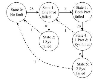
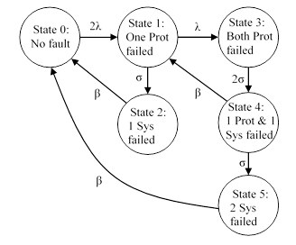
Consider two parallel systems, each with a built-in protection feature, and suppose the protection feature can fail latently at the constant rate λ. Once the protection has failed, the system is exposed to some unknown constant failure rate σ. In other words, with the protection failed, the mean time to system failure is 1/σ. This dual system is dispatched on a sequence of flights of duration T_f, and if either system fails, it is repaired prior to the next flight. Our objective is to determine the normalized average probability of both systems being failed on the same flight. The Markov model representation of this situation is depicted below.

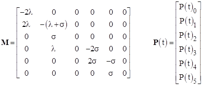
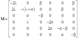
The transitions labeled with “1” are the discrete repair transitions that take place before each flight. The monotonic state equations for this model are dP/dt = MP, where

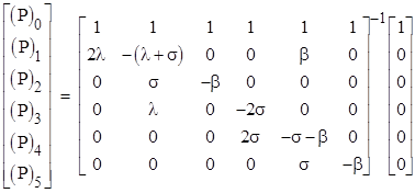
The probability state vector at the end of the kth flight is therefore given recursively by

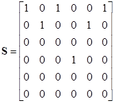
where the discrete repair transition matrix (sending the probability in States 1 and 5 back to State 0, and sending the probability in State 4 back to State 1) is

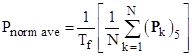
Given that the life of the airplane consists of N flights of duration T_f, the normalized average probability (also called “Average Probability per Flight Hour”) of State 5 as defined in the draft Arsenal AC 25.1309, is

For any given values of λ and σ we can compute the normalized probability, but our premise is that the value of σ is unknown. One might think that this makes it impossible to compute a useable probability, but in fact we can compute a robust upper bound on the probability by noting that the probability of State 5 would be zero if σ = 0, because in that case the systems would never fail, even if the protection features are failed. On the other hand, the probability of state 5 is also zero if σ is arbitrarily large, because in that case a system will fail almost immediately when its protection fails, so it will transition from State 1 immediately to State 2 and then back to State 0. Hence it can never reach States 3, 4, or 5. For values of σ between 0 and infinity, the probability of State 5 is positive, and it reaches a maximum at some value of σ. We can compute this upper bound on the probability of State 5, even though we do not know the actual value of σ.  (The same technique was discussed in the Section on Redundant Systems with a Common Threat.)

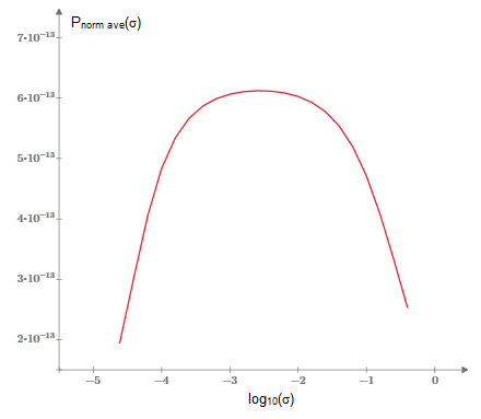
To illustrate, with λ = 2.63E-07/hr, the plot below shows the normalized average probability as a function of log(s).

From this we see that the maximum possible normalized average probability is about 6E-13/FH, which occurs with σ ≈ 10^−2.5.

An alternative approach is to approximate the discrete repair transitions with exponential repair transitions, and then evaluate the model in the steady-state condition to give the asymptotic average probability of State 5. The Markov model is as depicted below.

Here the repair transition is assigned the value β = 2/T_f, because the mean time between entering and exiting the state is half of the flight duration. The overall transition matrix is therefore

As discussed in “What is a Markov Model?”, the steady-state solution can be found by replacing one of the state equations (typically we choose the first) with the normalizing condition

Thus we have the steady-state solution

This gives the asymptotic probability of State 5 as

The so-called normalized average probability is given by dividing this by the average flight length T_f. Also, it should be noted that this expression averages throughout each flight, during which the probability in State 5 essentially increases linearly, so the probabilities at the end of the flights are twice the average. Hence the normalized average probability consistent with the draft Arsenal AC 25.1309 is the above expression multiplied by 2/T_f. For any given value of σ this gives the normalized average probability based on the steady-state (asymptotic) solution of the model with exponential repair transitions as

A plot of this function versus σ superimposed on the exact discrete solution is shown below.

Both of these gives essentially the same upper bound on the normalized average probability, i.e., about 6E-13/FH, but they differ appreciably for smaller values of σ. The reason for this is that for fairly large values of s the exact transient solution with discrete repairs reaches the steady-state condition during the life of the airplane, but for much smaller values of σ the system does not come close to reaching steady-state, so in the exact solution it is truncated at the life of the airplane. Thus for small s we would not expect the solutions to match unless we extend the life of the airplane by orders of magnitude. To illustrate, the plot below shows the two solutions, where the exact transient solution has been applied to 128 airplane life spans, which is how long it would take to approach steady-state.

This confirms that the two methods give consistent result, provided they are applied on an equal footing. Without knowing in advance whether a system will reach the steady-state condition, it is typically preferable to simply use the exact time-dependent solution. For airplane systems, an analysis of the failure rates for individual engines (for example) can generally use the steady-state approach, because the inflight failure rate of a fleet of engines will reach steady-state. In contrast, for the analysis of catastrophic conditions with such low probabilities that they are not expected to occur in the life of an airplane, the probability may never reach steady-state, if there are potential latent faults with unlimited exposures.

Return to MathPages Main Menu