7.6  Cosmological Coherence

Our main “difference in creed” is that you have a specific belief and I am a skeptic.

                                    Willem de Sitter to Einstein, 1917

Almost immediately after Einstein arrived at the final field equations of general relativity, the very foundation of his belief in those equations was shaken, first by appearance of Schwarzschild’s exact solution of the one-body problem. This was disturbing to Einstein because at the time he held the Machian belief that inertia must be attributable to the effects of distant matter, so he thought the only rigorous global solutions of the field equations would require some suitable distribution of distant matter. Schwarzschild’s solution represents a well-defined spacetime extending to infinity, with ordinary inertial behavior for infinitesimal test particles, even though the only significant matter in this universe is the single central gravitating body. That body influences the spacetime in its vicinity, but the metric throughout spacetime is primarily determined by the spherical symmetry, leading to asymptotically flat spacetime at great distances from the central body. This seems rather difficult to reconcile with “Mach’s Principle”, but there was worse to come, and it was Einstein himself who opened the door.

In an effort to conceive of a static cosmology with uniformly distributed matter he found it necessary to introduce another term to the field equations, with a coefficient called the cosmological constant. (See Section 5.8.) Shortly thereafter, Einstein received a letter from the astronomer Willem de Sitter, who pointed out a global solution of the modified field equations (i.e., with non-zero cosmological constant) that is entirely free of matter, and yet that possesses non-trivial metrical structure. This thoroughly un-Machian universe was a fore-runner of Gödel’s subsequent cosmological models containing closed-timelike curves. After a lively and interesting correspondence about the shape of the universe, carried on between a Dutch astronomer and a German physicist at the height of the first world war, de Sitter published a paper on his solution, and Einstein published a rebuttal, claiming (incorrectly) that “the De Sitter system does not look at all like a world free of matter, but rather like a world whose matter is concentrated entirely on the [boundary]”. The discussion was joined by several other prominent scientists, including Weyl, Klein, and Eddington, who all tried to clarify the distinction between singularities of the coordinates and actual singularities of the manifold/field. Ultimately all agreed that de Sitter was right, and his solution does indeed represent a matter-free universe consistent with the modified field equations.

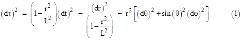
We’ve seen that the Schwarzschild metric represents the unique spherically symmetrical solution of the original field equations of general relativity − assuming the cosmological constant, denoted by λ in Section 5.8, is zero. If we allow a non-zero value of λ, the Schwarzschild solution generalizes to

To avoid upsetting the empirical successes of general relativity, such as the agreement with Mercury’s excess precession, the value of λ must be extremely small, certainly less than 10⁻⁴⁰ m⁻², but not necessarily zero. If λ is precisely zero, then the Schwarzschild metric goes over to the Minkowski metric when the gravitating mass m equals zero, but if λ is not precisely zero the Schwarzschild metric with zero mass is

where L is a characteristic length related to the cosmological constant by L² = 3/λ. This is one way of writing the metric of de Sitter spacetime. Just as Minkowski spacetime is a solution of the original vacuum field equations R_μν = 0, so the de Sitter metric is a solution of the modified field equations R_μν = λg_μν. Since there is no central mass in this case, it may seem un-relativistic to use polar coordinates centered on one particular point, but it can be shown that – just as with the Minkowski metric in polar coordinates – the metric takes the same form when centered on any point.

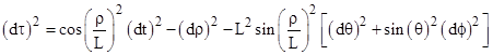
The metric (1) can be written in a slightly different form in terms of the radial coordinate ρ defined by

Noting that dr/L = cos(ρ/L)dρ, the de Sitter metric is

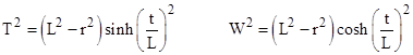
Interestingly, with a suitable change of coordinates, this is actually the metric of the surface of a four-dimensional pseudo-sphere in five-dimensional Minkowski space. Returning to equation (1), let x,y,z denote the usual three orthogonal spatial coordinates such that x² + y² + z² = r², and suppose there is another orthogonal spatial coordinate W and a time coordinate T defined by

For any values of x,y,z,t we have

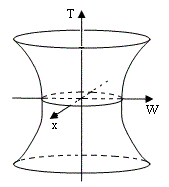
so this locus of events comprises the surface of a hyperboloid, i.e., a pseudo-sphere of “radius” L. In other words, the spatial universe for any given time T is the three-dimensional surface of the four-dimensional sphere of squared radius L² + T². Hence the space shrinks to a minimum radius L at time T = 0 and then expands again as T increases, as illustrated below (showing only two of the spatial dimensions).

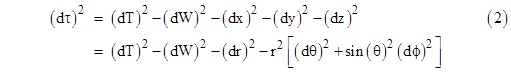
Assuming the five-dimensional spacetime x,y,z,W,T has the Minkowski metric

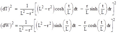
we can determine the metric on the hyperboloid surface by substituting the squared differentials (dT)² and (dW)²

into the five-dimensional metric, which gives equation (1). The accelerating expansion of the space for a positive cosmological constant can be regarded as a consequence of a universal repulsive force. The radius of the spatial sphere follows a hyperbolic trajectory similar to the worldlines of constant proper acceleration discussed in Section 2.9. To show that the expansion of the de Sitter spacetime can be seen as exponential, we can put the metric into the “Robertson-Walker form” (see Section 7.1) by defining a new system of coordinates  such that

where

It follows that

where

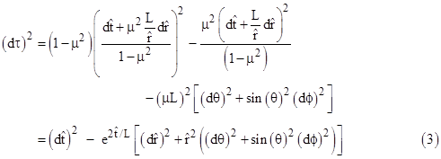
Substituting into the metric (1) gives the exponential form

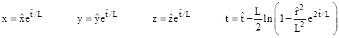
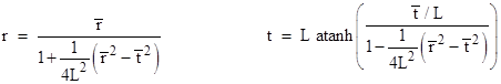
The characteristic length S(t) for this metric is the simple exponential function. (This form of the metric covers only part of the manifold.) Equations (1), (2), and (3) are the most common ways of expressing de Sitter’s metric, but in the first letter that de Sitter wrote to Einstein on this subject he didn’t give the line element in any of these familiar forms. We can derive his original formulation beginning with (1) if we define new coordinates  related to the r,t coordinates of (1) by

Incidentally, the t coordinate is the “relativistic difference” between the advanced and retarded combinations of the barred coordinates, i.e.,

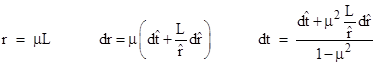
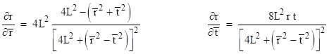
The differentials in (1) can be expressed in terms of the barred coordinates as

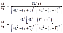
where the partials are

and

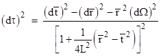
Making these substitutions and simplifying, we get the “Cartesian” form of the metric that de Sitter presented in his first letter to Einstein

where dΩ denotes the angular components, which are unchanged from (1). These expressions have some purely mathematical features of interest. For example, the line element is formally similar to the expressions for curvature discussed in Section 5.3. Also, the denominators of the partials of t are, according to Heron’s formula, equal to 16A² where A is the area of a triangle with edge lengths .

If the cosmological constant was zero (meaning that L was infinite) all the dynamic solutions of the field equations with matter predict a slowing rate of expansion, but in 1998 two independent groups of astronomers reported evidence that the expansion of the universe is actually accelerating. If these findings are correct, then some sort of repulsive force is needed in models based on general relativity. This has led to renewed interest in the possibility of a positive cosmological constant and de Sitter spacetime, which is sometimes denoted as dS₄. If the cosmological constant were negative, the resulting spacetime manifold would be anti-de Sitter spacetime, denoted by AdS₄. In the latter case, we would still get a hyperboloid, but the time coordinate advances circumferentially around the surface. To avoid closed time-like curves, we could simply imagine “wrapping” sheets around the hyperboloid.

As discussed in Section 7.1, the characteristic length S(t) of a manifold (i.e., the time-dependent coefficient of the spatial part of the manifold) satisfying the modified Einstein field equations (with non-zero cosmological constant λ) varies as a function of time in accord with the Friedmann equation

where dots signify derivatives with respect to a suitable time coordinate, C is a constant, and k is the curvature index, equal to −1, 0, or +1. The terms on the right hand side are akin to potentials, and it’s interesting to note that the first two terms correspond to the two hypothetical forms of gravitation highlighted by Newton in the Principia. (See Section 8.2 for more on this.) As explained in Section 7.1, the Friedmann equation implies that S satisfies

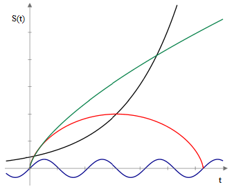
which shows that if λ = 0 the characteristic cosmological length S is a solution of the “separation equation” for non-rotating gravitationally governed distances as given by equation (3) of Section 4.2, leading to the familiar closed cycloidal solutions and asymptotically decelerating open solutions described in Section 7.1. On the other hand, for non-zero values of λ the equation has a much more diverse range of solutions, including sinusoidal and exponential functions. The latter can represent universes expanding at an accelerating rate, and hence can accommodate the 1998 observations. (It’s ironic that Einstein originally introduced this constant to reconcile the field equations with a static universe, whereas it is now used to reconcile them with an accelerating expansion of the universe.) A plot depicting some representative families of possible solutions to the field equations with non-zero λ is shown below.

Incidentally, if we were to set aside its connection with the field equations of general relativity, we might view the general cosmological scale equation as just a phenomenological equation, and compare it with the classical gravitational separation equation from Section 4.2. We have

This again highlights the inverse square and the direct proportionalities that caught Newton’s attention. Recall that with m = 0 the left-hand expression reduces to the purely inertial separation equation, and with λ = 0 the right hand expression reduces to the (non-rotating) gravitational separation equation. Both of these “homogeneous” equations are of the form  for some constant α, and solutions of this equation include the same families of sinusoidal and exponential solutions as in general relativity with non-zero λ. Of course, only α = 2 is consistent with the field equations of general relativity (in 3+1 dimensions), and hence the solutions with accelerating expansion in general relativity require a non-zero λ. Still, it’s interesting that, from a phenomenological perspective, we have this alternative “homogeneous” way of representing the wider range of solutions.

In this broader (and highly speculative) context, one could have been led, long before the recent astronomical observations, to imagine that there might be a class of exponential cosmological distances, not in place of, but in addition to the cycloidal and parabolic distances. In other words, there could be different classes of observable distances on various scales, some very small and oscillatory, some larger and slowing, and some – the largest of all – increasing at an accelerating rate, as illustrated in the figure above.

Naturally, according to all conventional metrical theories, including general relativity, the spatial relations between material objects (on any chosen temporal foliation) conform to a single three-dimensional manifold. Assuming homogeneity and isotropy, it follows that all the cosmological distances between objects are subject to the ordinary metrical relations such as the triangle inequality. This greatly restricts the observable distances. On the other hand, our assumption that the degrees of freedom are limited in this way (for three dimensional space) is based on our experience with much smaller distances. We have no direct evidence that cosmological distances are subject to the same dependencies. As an example of how concepts based on limited experience can be misleading, recall how special relativity revealed that the “metric” of our local spacetime fails to satisfy the axioms of a metric, including the triangle inequality. The non-additivity of relative speeds was not anticipated based on human experience with low speeds. Likewise for three “co-linear” objects A,B,C, it’s conceivable that the distance AC is not the simple sum of the distances AB and BC. The feasibility of regarding separations (rather than particles) as the elementary objects of nature was discussed in Section 4.1.

One possible observational consequence of having distances of several different classes would be astronomical objects that are highly red-shifted and yet much closer to us than the standard Hubble model would imply based on their redshifts. (Of course, even if this view was correct, it might be the case that all the exponential separations have already passed out of view.) Another possible consequence would be that some observable distances would be increasing at an accelerating rate, whereas others of the same magnitude might be decelerating.

This discussion is just intended to show that the idea of at least some cosmological separations increasing at an accelerating rate can arise from completely a priori considerations, and that we need not even assume that cosmological distances are consistent with a single coherent three-dimensional manifold. Nevertheless, as long as a single coherent expansion model is adequate to explain our observations, the standard general relativity models of a smooth manifold remain the best supported models. Less conventional notions such as those discussed above would be called for only if we begin to see conflicting evidence, e.g., if some observed distances indicated accelerating expansion while others indicated decelerating expansion.

As mentioned in Section 7.1., George Gamow reported that Einstein regarded the introduction of the cosmological constant as his “biggest blunder”, but there are differing views as to why he might have regarded it as a “blunder”. Some have suggested that Einstein was annoyed by his failure to see the dynamical solutions of the field equations, and thereby missing the opportunity to predict the Hubble expansion. However, in his own writings, Einstein argued that “the introduction of [the cosmological constant] constitutes a complication of the theory, which seriously reduces its logical simplicity”. He also wrote “If there is no quasi-static world, then away with the cosmological term”, adding that it is “theoretically unsatisfactory anyway”. In modern usage the cosmological term is usually taken to characterize some feature of the vacuum state, so it is a fore-runner of the extremely complicated vacua that are contemplated in the “string theory” research program. If Einstein considered the complication and loss of logical simplicity associated with a single constant to be theoretically unsatisfactory, he might have been even more dissatisfied with the nearly infinite number of possible vacua contemplated in current string research. Oddly enough, the anti-de Sitter spacetimes play a prominent role in this research, especially in relation to the so-called AdS/CFT conjecture involving conformal field theory.

Return to Table of Contents