9.3  Higher-Order Metrics

A similar path to the same goal could also be taken in those manifolds in which the line element is expressed in a less simple way, e.g., by a fourth root of a differential expression of the fourth degree…

                                                  Riemann, 1854

Given three points A,B,C, let dx¹ denote the distance between A and B, and let dx² denote the distance between B and C. Can we express the distance ds between A and C in terms of dx¹ and dx²? Since dx¹, dx², and ds all represent distances with commensurate units, it's clear that any formula relating them must be homogeneous in these quantities, i.e., they must appear to the same power. One possibility is to assume that ds is a linear combination of dx¹ and dx² as follows

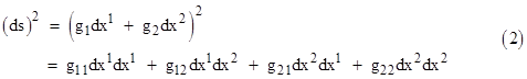
where g₁ and g₂ are constants. In a simple one-dimensional manifold this would indeed be the correct formula for ds, with |g₁| = |g₂| = 1, except for the fact that it might give a negative sign for ds, contrary to the idea of an interval as a positive magnitude. To ensure the correct sign for ds, we might take the absolute value of the right hand side, which suggests that the fundamental equality actually involves the squares of the two sides of the above equation, i.e., the quantities ds, dx¹, dx² satisfy the relation

where we have put g_ij = g_i g_j. Thus we have g₁₁g₂₂ − 4(g₁₂)² = 0, which is the condition for factorability of the expanded form as the square of a linear expression. This will be the case in a one-dimensional manifold, but in more general circumstances we find that the values of the g_ij in the expanded form of (2) are such that the expression is not factorable into linear terms with real coefficients. In this way we arrive at the second-order metric form, which is the basis of Riemannian geometry.

Of course, by allowing the second-order coefficients g_ij to be arbitrary, we make it possible for (ds)² to be negative, analogous to the fact that ds in equation (1) could be negative, which is what prompted us to square both sides of (1), leading to equation (2). Now that (ds)² can be negative, we're naturally led to consider the possibility that the fundamental relation is actually the equality of the squares of both sides of (2). This gives

where the sum is evaluated for μ,ν,α,β each ranging from 1 to n, where n is the dimension of the manifold. Once again, having arrived at this form, we immediately dispense with the assumption of factorability, and allow general fourth-order metrics. These are non-Riemannian metrics, although Riemann actually alluded to the possibility of fourth and higher order metrics in his famous inaugural dissertation. He noted that

The line element in this more general case would not be reducible to the square root of a quadratic sum of differential expressions, and therefore in the expression for the square of the line element the deviation from flatness would be an infinitely small quantity of degree two, whereas for the former manifolds [i.e., those whose squared line elements are sums of squares] it was an infinitely small quantity of degree four. This peculiarity [i.e., this quantity of the second degree] in the latter manifolds therefore might well be called the planeness in the smallest parts…

It's clear even from his brief comments that he had given this possibility considerable thought, but he never published any extensive work on it. Finsler wrote a dissertation on this subject in 1918, so such metrics are now often called Finsler metrics.

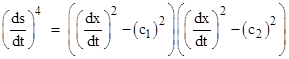
To visualize the effect of higher order metrics, recall that for a second-order metric the locus of points at a fixed distance ds from the origin must be a conic, i.e., an ellipse, hyperbola, or parabola. In contrast, a fourth-order metric allows more complicated loci of equi-distant points. When applied in the context of Minkowskian metrics, these higher-order forms raise some intriguing possibilities. For example, instead of a spacetime structure with a single light-like characteristic c, we could imagine a structure with two null characteristics, c₁ and c₂. Letting x and t denote the spacelike and timelike coordinates respectively, this means (ds/dt)⁴ vanishes for two values (up to sign) of dx/dt. Thus there are four roots given by ±c₁ and ±c₂, and we have

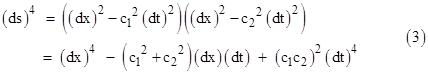
The resulting metric is

The physical significance of this "metric" naturally depends on the physical meaning of the coordinates x and t. In Minkowski spacetime these represent what physical rulers and clocks measure, and we can translate these coordinates from one inertial system to another according to the Lorentz transformations while always preserving the form of the Minkowski metric with a fixed numerical value of c. The coordinates x and t are defined in such a way that c remains invariant, and this definition happily coincides with the physical measures of rulers and clocks. However, with two distinct light-like "eigenvalues", it's no longer possible for a single family of spacetime decompositions to preserve the values of both c₁ and c₂. Consequently, the metric will take the form of (3) only with respect to one particular system of xt coordinates. In any other frame of reference at least one of c₁ and c₂ must be different.

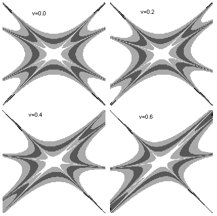
Suppose that with respect to a particular inertial system of coordinates x,t the spacetime metric is given by (3) with c₁ = 1 and c₂ = 2. We might also suppose that c₁ corresponds to the null surfaces of electromagnetic wave propagation, just as in Minkowski spacetime. Now, with respect to any other system of coordinates x′,t′ moving with speed v relative to the x,t coordinates, we can decompose the absolute intervals into space and time components such that c₁ = 1, but then the values of the other lightlines (corresponding to ±c₂′) must be (v+c₂)/(1+vc₂) and (v−c₂)/(1−vc₂). Consequently, for states of motion far from the one in which the metric takes the special form (3), the metric will become progressively more asymmetrical. This is illustrated in the figure below, which shows contours of constant magnitude of the squared interval.

Clearly this metric does not correspond to the observed spacetime structure, even in the symmetrical case with v = 0, because it is not Lorentz-invariant. As an alternative to this structure containing "super-light" null surfaces we might consider metrics with some finite number of "sub-light" null surfaces, but the failure to exhibit even approximate Lorentz-invariance would remain.

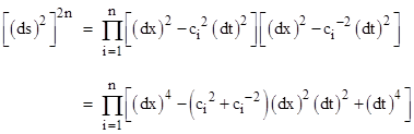
However, it is possible to construct infinite-order metrics with infinitely many super-light and/or sub-light null surfaces, and in so doing recover a structure that in many respect is virtually identical to Minkowski spacetime, except for a set (of spacetime trajectories) of measure zero. This can be done by generalizing (3) to include infinitely many discrete factors

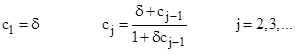
where the values of c_i represent an infinite family of sub-light parameters given by

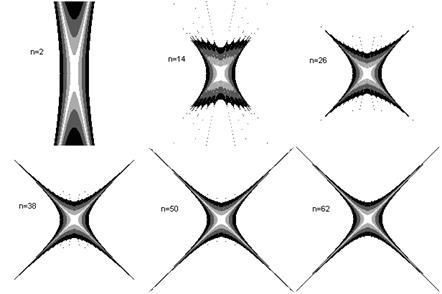
for some constant δ. A plot showing how this spacetime structure develops as n increases is shown below.

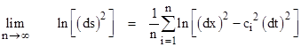
This illustrates how, as the number of sub-light cones goes to infinity, the structure of the manifold goes over to the usual Minkowski pseudometric, except for the discrete null sub-light surfaces which are distributed throughout the interior of the future and past light cones, and which accumulate on the light cones. The sub-light null surfaces become so thin that they no linger show up on these contour plots for large n, but they remain present to all orders. In the limit as n approaches infinity they become discrete null trajectories embedded in what amounts to ordinary Minkowski spacetime. To see this, notice that if none of the factors on the right hand side of (4) is exactly zero we can take the natural log of both sides to give

Thus the natural log of (ds)² is the asymptotic average of the natural logs of the quantities (dx)² − c_i²(dt)². Since the values of c_i accumultate on 1, it's clear that this converges on the usual Minkowski metric (provided we are not precisely on any of the discrete sub-light null surfaces).

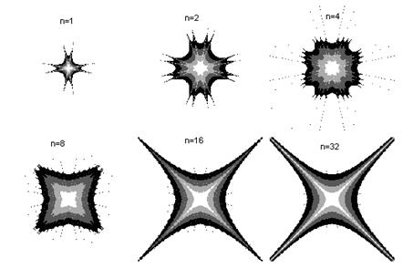
The preceding metric was based purely on sub-light null surfaces. We could also include n super-light null surfaces along with the n sub-light null surfaces, yielding an asymptotic family of metrics which, again, goes over to the usual Minkowski metric as n goes to infinity (except for the discrete null surface structure). This metric is given by the formula

where the values of c_i are generated as before. The results for various values of n are illustrated in the figure below.

Notice that the quasi Lorentz-invariance of this metric has a subtle periodicity, because any one of the sublight null surfaces can be aligned with the time axis by a suitable choice of velocity, or the time axis can be placed "in between" two null surfaces. In a 1+1 dimensional spacetime the structure is perfectly symmetrical modulo this cycle from one null surface to the next. In other words, the set of exactly equivalent reference systems corresponds to a cycle with a period of δ, which is the increment between each c_i and c_i+1. However, with more spatial dimensions the sub-light null structure is subtly less symmetrical, because each null surface represents a discrete cone, which associates two of the trajectories in the xt plane as the sides of a single cone. Thus there must be an absolutely innermost cone, in the topological sense, even though that cone may be far off center, i.e., far from the selected time axis. Similarly for the super-light cones (or spheres), there would be a single state of motion with respect to which all of those null surfaces would be spherically symmetrical. Only the accumulation shell, i.e., the actual light-cone itself, would be spherically symmetrical with respect to all states of motion.

Return to Table of Contents