9.5  Entangled Events

Anyone who is not shocked by quantum theory has not understood it.

                                       Niels Bohr, 1927

A paper written by Einstein, Podalsky, and Rosen (EPR) in 1935 described a thought experiment which, the authors believed, demonstrated that quantum mechanics does not provide a complete description of physical reality, at least not if we accept certain common notions of locality and realism. Subsequently the EPR experiment was refined by David Bohm (so it is now called the EPRB experiment) and analyzed in detail by John Bell, who highlighted a fascinating subtlety that Einstein, et al, may have missed. Bell showed that the outcomes of the EPRB experiment predicted by quantum mechanics are inherently incompatible with conventional notions of locality and realism combined with a certain set of assumptions about causality. The precise nature of these causality assumptions is rather subtle, and Bell found it necessary to revise and clarify his premises from one paper to the next. In Section 9.6 we discuss Bell's assumptions in detail, but for the moment we'll focus on the EPRB experiment itself, and the outcomes predicted by quantum mechanics.

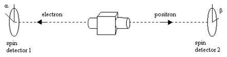
Most actual EPRB experiments are conducted with photons, but in principle the experiment could be performed with massive particles. The essential features of the experiment are independent of the kind of particle we use. For simplicity we'll describe a hypothetical experiment using electrons (although in practice it may not be feasible to actually perform the necessary measurements on individual electrons). Consider the decay of a spin-0 particle resulting in two spin-1/2 particles, an electron and a positron, ejected in opposite directions. If spin measurements are then performed on the two individual particles, the correlation between the two results is found to depend on the difference between the two measurement angles. This situation is illustrated below, with α and β signifying the respective measurement angles at detectors 1 and 2.

Needless to say, the mere existence of a correlation between the measurements on these two particles is not at all surprising. In fact, this would be expected in most classical models, as would a variation in the correlation as a function of the absolute difference θ = |α – β| between the two measurement angles. The essential strangeness of the quantum mechanical prediction is not the mere existence of a correlation that varies with θ, it is the non-linearity of the predicted variation.

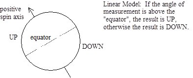
If the correlation varied linearly as θ ranged from 0 to π, it would be easy to explain in classical terms. We could simply imagine that the decay of the original spin-0 particle produced a pair of particles with spin vectors pointing oppositely along some randomly chosen axis. Then we could imagine that a measurement taken at any particular angle gives the result UP if the angle is within π/2 of the positive spin axis, and gives the result DOWN otherwise. This situation is illustrated below:

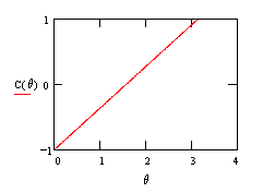
Since the spin axis is random, each measurement will have an equal probability of being UP or DOWN. In addition, if the measurements on the two particles are taken in exactly the same direction, they will always give opposite results (UP/DOWN or DOWN/UP), and if they are taken in the exact opposite directions they will always give equal results (UP/UP or DOWN/DOWN). Also, if they are taken at right angles to each other the results will be completely uncorrelated, meaning they are equally likely to agree or disagree. In general, if θ denotes the absolute value of the angle between the two spin measurements, the above model implies that the correlation between these two measurements would be C(θ) = (2/π)θ – 1, as plotted below.

This linear correlation function is consistent with quantum mechanics (and confirmed by experiment) if the two measurement angles differ by θ = 0, π/2, or π, giving the correlations –1, 0, and +1 respectively.

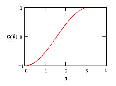
However, for intermediate angles, quantum theory predicts (and experiments confirm) that the actual correlation function for spin-1/2 particles is not the linear function shown above, but the non-linear function given by C(θ) = –cos(θ), as shown below

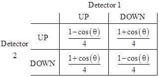
On this basis, the probabilities of the four possible joint outcomes of spin measurements performed at angles differing by θ are as shown in the table below. (The same table would apply to spin-1 particles such as photons if we replace θ with 2θ.)

To understand why these correlations defy explanation within the classical framework of local realism, suppose we confine ourselves to spin measurements along one of just three axes, at 0, 120, and 240 degrees. Several pairs of entangled particles are produced and sent off to two distant locations in opposite directions. In both locations a spin measurement along one of the three established axes is performed, and the results are recorded. The choices of measurements (0°, 120°, or 240°) at each detector may be arbitrary, e.g., by flipping coins, or by any other means. In each location it is found that, regardless of which measurement is made, there is an equal probability of spin UP or spin DOWN. This is all that the experimenters at either site can determine separately.

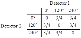
However, when all the results are brought together and compared in matched pairs, we find the following joint correlations

The numbers in this matrix indicate the fraction of times that the results agreed (both UP or both DOWN) when the indicated measurements were made on the two members of a matched pair of objects. Notice that if the two distant experimenters happened to measure the spin along the same direction for a given pair of particles, the results never agreed, i.e., they always exhibited opposite spin (one UP and one DOWN). Also notice that, if both measurement angles are selected at random, the overall probability of agreement is 1/2.

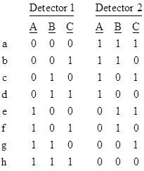
The remarkable fact is that there is no way, within the traditional view of physical processes, to account for the joint probabilities listed above. To see why, notice that if a particle at Detector 1 is measured in direction 0° and yields spin UP, then the corresponding particle at Detector 2 must yield spin DOWN if measured in direction 0°. Now, assuming the particles and measurements at the two detectors are completely separable, we must conclude that this particle at Detector 2 will yield spin DOWN regardless of whether the other particle is measured in the 0° direction or not. Thus each particle must be prepared to respond in a definite way to any one of the three measurements. This, in itself, would not be difficult to understand classically, since we could simply assume that some “hidden variables” carried by the particles determine the outcomes of spin measurements, and these are assigned when the entangled pairs are produced so that they yield perfect anti-correlation when measured along the same direction. But this turns out to be impossible to reconcile with the correlations for pairs measured at unequal angles. To see why, consider the eight possible ways of preparing a pair of particles:

Here “0” and “1” signify the particle will yield spin DOWN and UP respectively. These preparations, and only these, will yield the required anti-correlation when the particles are measured in the same direction. Therefore, each pair of entangled particles must be pre-programmed (at the moment when they separate from each other) in one of the eight ways shown above. It only remains now to determine the probabilities of these eight preparations.

The simplest state of affairs would be for each of the eight possible preparations to be equally probable (each with probability 1/8), but in that case the probability of agreement for unequal measurement angles (the off-diagonal cells in the preceding table) would be just 1/2, and the overall probability of agreement for random measurement angles would be just 1/3, so that possibility is ruled out. Even if we assume the probabilities of the pair types ‘a’ and ‘h’ are zero and the remaining six kinds of pairs each have probability 1/6, the probabilities of agreement for unequal measurement angles would be just 2/3 (instead of 3/4), and would give only 4/9 (instead of 1/2) for the overall probability of agreement for randomly chosen measurement angles.

Now, we might think some other weighting of these eight preparation states will give the right overall results, but in fact no such weighting is possible. The overall preparation process must yield some linear convex combination of the eight mutually exclusive cases, i.e., each of the eight possible preparations must have some fixed long-term probability, which we will denote by a, b,.., h, respectively. These probabilities are all positive values in the range 0 to 1, and the sum of these eight values is identically 1. It follows that the sum of the six probabilities b through g must be less than or equal to 1. This is a simple form of "Bell's inequality", which must be satisfied by any local realistic model of the sort that Bell had in mind. However, according to quantum mechanics, the probability of agreement when the spins are measured at unequal angles is 3/4, and by considering the cases when measurements at A and B agree, and at B and C, and at C and A, we have respectively

Adding these three expressions together gives 2(b + c + d + e + f + g) = 9/4, so the sum of the probabilities b through g is 9/8, which exceeds 1. Hence the results of the EPRB experiment predicted by quantum mechanics (and empirically confirmed) violate Bell's inequality. This shows that there does not exist a linear combination of those eight preparations that can yield the joint probabilities predicted by quantum mechanics, so there is no way of accounting for the actual experimental results by means of any realistic local physical model of the sort that Bell had in mind. The observed violations of Bell's inequality in EPRB experiments imply that Bell's conception of “local realism” is inadequate to represent the actual processes of nature.

The causality assumptions underlying Bell's analysis are inherently problematic (see Section 9.7), but the analysis is still important, because it highlights the fundamental inconsistency between the predictions of quantum mechanics and certain conventional ideas about causality and local realism. In order to maintain those conventional ideas, we might suppose that information about the choice of measurement basis at one detector is somehow conveyed to the other detector, influencing the outcome at that detector, even though the measurement events are space-like separated. For this reason, some people have been tempted to think that violations of Bell's inequality imply superluminal communication, contradicting the principles of special relativity. However, there is actually no effective transfer of information from one measurement to the other in an EPRB experiment, so the principles of special relativity are safe. One of the most intriguing aspects of Bell's analysis is that it shows how the workings of quantum mechanics (and, evidently, nature) involve correlations between space-like separated events that seemingly could only be explained by the presence of information from distant locations, even though the separate events themselves give no way of inferring that information. In the abstract, this is similar to "zero-information proofs" in mathematics.

To illustrate, consider a "twins paradox" involving a pair of twin brothers who are separated and sent off to distant locations in opposite directions. When twin #1 reaches his destination he asks a stranger there to choose a number x₁ from 1 to 10, and the twin writes this number down on a slip of paper along with another number y₁ of his own choosing. Likewise twin #2 asks someone at his destination to choose a number x₂, and he writes this number down along with a number y₂ of his own choosing. When the twins are re-united, we compare their slips of paper and find that |y₂ – y₁| = (x₂ – x₁)². This is really astonishing. Of course, if the correlation was some linear relationship of the form y₂ – y₁ = A(x₂ – x₁) + B for any pre-established constants A and B, the result would be quite easy to explain. We would simply surmise that the twins had agreed in advance that twin #1 would write down y₁ = Ax₁ – B/2, and twin #2 would write down y₂ = Ax₂ + B/2. However, no such explanation is possible for the observed non-linear relationship, because there do not exist functions f₁ and f₂ such that f₂(x₂) – f₁(x₁) = (x₂ – x₁)². Thus if we assume the numbers x₁ and x₂ are independently and freely selected, and there is no communication between the twins after they are separated, then there is no "locally realistic" way of accounting for this non-linear correlation. It seems as though one or both of the twins must have had knowledge of his brother's numbers when writing down his own number, despite the fact that it is not possible to infer anything about the individual values of x₂ and y₂ from the values of x₁ and y₁ or vice versa.

In the same way, the results of EPRB experiments imply a greater degree of inter-dependence between separate events than can be accounted for by traditional models of causality. One possible idea for adjusting our conceptual models to accommodate this aspect of quantum phenomena would be to deny the existence of any correlations until they becomes observable. According to the most radical form of this proposal, the universe is naturally partitioned into causally compact cells, and only when these cells interact do their respective measurement bases become reconciled, in such a way as to yield the quantum mechanical correlations. This is an appealing idea in many ways, but it's far from clear how it could be turned into a realistic model. Another possibility is that the preparation of the two particles at the emitter and the choices of measurement bases at the detectors may be mutually influenced by some common antecedent event(s). This can never be ruled out, as discussed in Section 9.6. Lastly, we mention the possibility that the preparation of the two particles may be conditioned by the measurements to which they are subjected. This is discussed in Section 9.9.

Return to Table of Contents