Weibull Analysis

Given any function g(x) with g(0) = 0 and increasing monotonically to infinity as x goes to infinity, we can define a cumulative probability function by

Obviously this probability is 0 at t = 0 and increases monotonically to 1.0 as t goes to infinity. The corresponding density distribution f(t) is the derivative of this, i.e.,

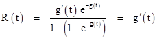
As discussed in Failure Rates, MTBFs, and All That, the "rate" of occurrence for a given density distribution is

so the rate for the preceding density function f(t) is

This enables us to define a probability density distribution with any specified rate function R(t). One useful two-parameter family of rate functions is given by

where η and β are constants (pronounced eta and beta). This is the so-called "Weibull" family of distributions, named after the Swedish engineer Waloddi Weibull (1887-1979) who popularized its use for reliability analysis, especially for metallurgical failure modes. Weibull's first paper on the subject was published in 1939, but the method didn't attract much attention until the 1950's. Interestingly, the "Weibull distribution" had already been studied in the 1920's by the statistician Emil Gumbel (1891-1966), who is best remembered today for his confrontation with the Nazis in 1931 when they organized a campaign to force him out of his professorship at Heidelberg University for his outspoken pacifist and anti-Nazi views.

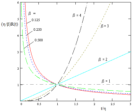
The constant η is called the scale parameter, because it scales the t variable, and the constant β is called the shape parameter, because it determines the shape of the rate function. (Occasionally the variable t in the above definition is replaced with t−γ, where γ is a third parameter, used to define a suitable zero point.) If β is greater than 1 the rate increases with t, whereas if β is less than 1 the rate decreases with t. If β = 1 the rate is constant, in which case the Weibull distribution equals the exponential distribution. The shapes of the rate functions for the Weibull family of distributions are illustrated in the figure below

Since R(t) equals g'(t), we integrate this function to give

Clearly for any positive η and β parameters the function g(t) monotonically increases from 0 to infinity as t increases from 0 to infinity, so it yields a valid cumulative density distribution, namely

and the corresponding density distribution is

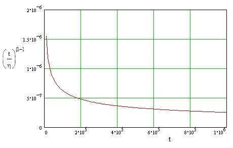
Suppose we have a population consisting of n widgets (where n is a large number), all of which began operating continuously at the same time t = 0. (Note that this time variable t represents "calendar time", which is the hours of operation of each individual widget, not the sum total of the operational hours of the entire population; the latter would be given by nt. We can use a single t as the time variable because we've assumed a coherent population consisting of widgets that began operating at the same instant and accumulated hours continuously. We defer the discussion of non-coherent populations until later.) If each widget has a Weibull cumulative failure distribution given by equation (2) for some fixed parameters η and β, then the expected number N(t) of failures by the time t is

Dividing both sides by n, and re-arranging terms, this can be written in the form

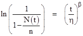
Taking the natural log of both sides and negating both sides, we have

Taking the natural log again, we arrive at

If the number N(t) of failures is very small compared with the total number n of widgets, the inner natural log on the left hand side can be approximated by the first-order term of the power series expansion, which gives simply N(t)/n, so we have

However, it's usually just as easy to use the exact equation (5) rather than the approximate equation (6).

Given an initial population of n = 100 widgets beginning at time t = 0, and accumulating hours continuously thereafter, suppose the first failure occurs at time t = t₁. Roughly speaking, we could say the expected number of failures at the time of the first failure is about 1, so we could put F(t₁) = N(t₁)/n = 1/100. However, this isn't quite optimum, because statistically the first failure is most likely to occur slightly before the expected number of failures reaches 1. To understand why, consider a population consisting of just a single widget, in which case the expected number of failures at any given time t would be simply F(t), which only approaches 1 in the limit as t goes to infinity, and yet the median time of failure is at the value of t = t_median such that F(t_median) = 0.5. In other words, the probability is 0.5 that the failure will occur prior to t_median, and 0.5 that it will occur later. Hence in a population of size n = 1 the expected number of failures at the median time of the first failure is just 0.5.

In general, given a population of n widgets, each with the same failure density f(t), the probability for each individual widget being failed at time t_m is F(t_m) = N(t_m)/n. Denoting this value by ϕ, the probability that exactly j widgets are failed and n - j are not failed at time t_m is

It follows that the probability of j or more being failed at the time t_m is

This represents the probability that the jth (of n) failure has occurred by the time t_m, and of course the complement is the probability that the jth failure has not yet occurred by the time t_m. Therefore, given that the jth failure occurs at t_m, the "median" value of F(t_m) = f is given by putting P[³j;n] = 0.5 in the above equation and solving for f. This value is called the median rank, and can be computed numerically. An alternative approach is to use the remarkably good approximate formula

This is the value (rather than j/n) that should be assigned to N(t_j)/n for the jth failure.

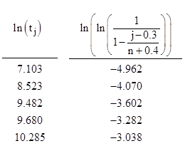
To illustrate, consider again an initial population of n = 100 widgets beginning at time t = 0, and accumulating hours continuously thereafter, and suppose the first five widget failures occurred at the times t₁ = 1216 hours, t₂ = 5029 hours, t₃ = 13125 hours, t₄ = 15987 hours, and t₅ = 29301 hours. This gives us five data points

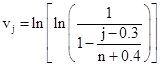
By simple linear regression we can perform a least-squares fit of this sequence of k = 5 data points to a line. In terms of variables x_j = ln(t_j) and

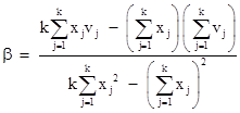
the estimated Weibull parameters are given by

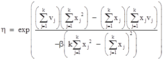
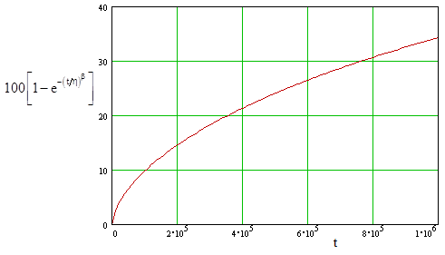
For our example with k = 5 data points, we get β = 0.609 and η = (4.14)10⁶ hours. Using equation (4), we can then forecast the expected number of failures into the future, as shown in the figured below.

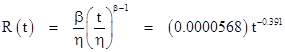
Notice that at the time t = η we expect 63.21% of the population to have failed, regardless of the value of β. The estimated failure rate for each individual widget as a function of time is

This function is shown in the figure below.

A distribution of this kind is said to exhibit an "infant mortality" characteristic, because the failure rate is initially very high, and then drops off.

For an alternative derivation of equation (6) for small N(t)/n, notice that the overall failure rate for the whole population of n widgets in essentially nR(t) because the number of functioning widgets does not change much as long as N(t)/n is small. Therefore, the expected number of failures by the time T for a coherent population of n widgets is

Dividing both sides by n and taking the natural log of both sides gives, again, equation (6). However, it should be noted that this applies only for times t such that N(t) is small compared with n. This is because we are analyzing the failure rate without replacement, so the value of n (the size of the unfailed population) is actually decreasing with time. By limiting our considerations to small values of N(t) (compared with n) we make this effect negligible. Now, it might seem that we could just as well assume replacement of the failed units, so that the size of the overall population remains constant, and indeed this is typically how analyses are conducted for devices with exponential failure distributions, for which the failure rate is constant. However, for the Weibull distribution it is not so easy, because the failure rate of each widget is a function of the age of that particular widget. If we replace a unit that has failed at 10000 hours with a new unit, the overall failure rate of the total population changes abruptly, either up or down, depending on whether β is less than or greater than 1.

The dependence of the failure rate R(t) on the time of each individual widget is also the reason we considered a coherent population of widgets whose ages are all synchronized. The greatly simplifies the analysis. In more realistic situations the population of widgets will be changing, and the "age" of each widget in the population will be different, as will the rate at which it accumulates operational hours as a function of calendar time. More generally we could consider a population of widgets such that each widget has it's own "proper time" τ_j given by τ_j = μ_j(t - γ_j) for all t greater than γ_j, where t is calendar time, γ_j is the birth date of the jth widget, and μ_j is the operational usage factor. This proper time is then the time variable for the Weibull density function for the jth widget, and the overall failure rate for the whole population at any given calendar time is composed of all the individual failure rates. In this non-coherent population, each widget has its own distinct failure distribution.

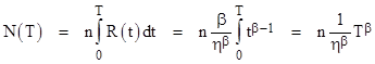
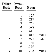
At a given calendar time, the experience basis of a particular population of n=10 total widgets might be as illustrated below:

So far there have been three failures, widgets 2, 4, and 5. The other seven widgets are continuing to accumulate operational hours at their respective rates. These are sometimes called "right censured" data points, or "suspensions", because we imagine that the testing has been suspended on these seven units prior to failure. We don't know when they will fail, so we can't directly use them as data points to fit the distribution, but we would still like to make some use of the fact that they accumulated their respective hours without failure. The usual approach in reliability analysis is to first rank all the data points according to their accumulated hours, as shown below.

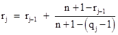
Next we assign adjust ranks to the widgets that have actually failed. Letting q_j denote the overall rank of the jth failure, and letting r_j denote the adjusted rank of the jth failure (with r₀ defined as 0), the adjusted rank of the jth failure is given by the formula

So, for the example above, we have

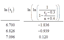
Using these adjusted ranks, we have the three data points

Fitting these three points using linear regression (as discussed above), we get the Weibull parameters η = 1164 and β = 4.767. The expected number of failures (which is just n times the cumulative distribution function) is shown below.

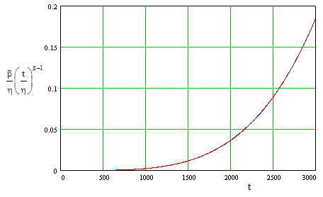
This shows a clear "wear out" characteristic, consistent with the observed failures (and survivals). The failure rate is quite low until the unit reaches about 500 hours, at which point the rate begins to increase, as shown in the figure below.

The examples discussed above are classical applications of the Weibull distribution, but the Weibull distribution is also sometimes used more loosely to model the "maturing system" effect of a high level system being introduced into service. In such a context the variation in the failure rate is attributed to gradual increase in familiarity of the operators with the system, improvements in maintenance, incorporation of retro-fit modifications to the design or manufacturing processes to fix unforeseen problems, and so on. Whether the Weibull distribution is strictly suitable to model such effects is questionable, but it seems to have become an accepted practice. In such applications it is common to lump all the accumulated hours of the entire population together, as if every operating unit has the same failure rate at any given time. This makes the analysis fairly easy, since it avoids the need to consider "censored" data, but, again, the validity of this assumption is questionable.

Return to MathPages Main Menu