Did Newton Answer Halley’s Question?

One of the most famous and consequential meetings in the history of science took place in the summer of 1684 when the young astronomer Edmund Halley paid a visit to Isaac Newton, during which Halley asked Newton what path a planet would follow if it were attracted toward the sun by a force proportional to the reciprocal of the squared distance. The idea that the planets were attracted to the sun by such an “inverse-square” force law had by then occurred to several people, including the architect Christopher Wren, the scientist Robert Hooke, and to Newton himself, following the publication by Huygens of the expression F = mω²r for the “centrifugal (outward) force” of a particle of mass m moving in a circular path of radius r with angular speed ω. This is equivalent to Kepler’s third law, which may be expressed as M = ω²r³, if we equate the outward “force” on a planet of mass m with the inward force of attraction toward the sun of magnitude F = Mm/r², where M is the mass of the sun (in suitable units so that G = 1). Of course, at the time, the constant M in Kepler’s third law was not known to be the mass of the sun, but it was clear that if both Huygens’s law of centrifugal force and Kepler’s third law were to be satisfied for circular orbits, the force of attraction must be proportional to the reciprocal of the square of the distance. Furthermore, it isn’t hard to see (from the modern Newtonian perspective) that Kepler’s second law, stating that a planet sweeps out equal areas in equal times, will automatically be satisfied given only that the force of attraction is always directly towards the sun, i.e., given a “central force”. This leaves unconfirmed only Kepler’s first law, which states that the planets move in elliptical paths with the sun at one of the focal points. Wren, Hooke, and Halley had discussed the problem at a coffee house following a meeting of the Royal Society in January of 1684, and Wren had offered a cash prize to whoever could provide a derivation of the shape of planetary orbits under the assumption of an inverse-square central force of attraction toward the (presumed stationary) sun. Hooke had claimed to have a proof that the paths were ellipses, but never provided it. Against this background, Halley paid a visit to Newton, who later told Abraham De Moivre about the fateful meeting. According to De Moivre

In 1684 Dr Halley came to visit him at Cambridge. After they had been some time together, the Dr asked him what he thought the curve would be that would be described by the planets supposing the force of attraction towards the sun to be reciprocal to the square of their distance from it. Sir Isaac replied immediately that it would be an ellipse. The Doctor, struck with joy and amazement, asked him how he knew it. Why, saith he, I have calculated it. Whereupon Dr Halley asked him for his calculation without any farther delay. Sir Isaac looked among his papers but could not find it, but he promised him to renew it and then to send it him…

As is well known, Halley’s question prompted Newton to formulate his ideas about mechanics and universal gravitation. The answer to Halley grew and became progressively more comprehensive until, in a remarkably short time (about 18 months), Newton had composed the three-volume work entitled The Mathematical Principles of Natural Philosophy, usually called by the Latin title “Philosophiae Naturalis Principia Mathematica”, or simply “Principia”, comprising the foundation of modern physics. It represents arguably the greatest single advance in human understanding ever achieved in the history of science. Just two months after its publication, the mathematician David Gregory wrote a letter to Newton, saying

Having seen and read your book I think my self obliged to give you my most hearty thanks for having been at the pains to teach the world that which I never expected any man should have known. For such is the mighty improvement made by you in the geometry, and so unexpectedly successful the application thereof to the physics, that you justly deserve the admiration of the best Geometers and Naturalists, in this and all succeeding ages.

And yet, it’s a curious fact that when the Principia was published (at Halley’s expense) in 1687, it did not actually contain the demonstration that Halley had requested. In a careful series of propositions (11 to 13 of Book 1), the Principia shows that a planet moving in a conical orbit under the influence of a central force toward one of the foci is undergoing acceleration toward that foci with a magnitude proportional to the reciprocal of the squared distance, and hence is subject to an inverse-square force. This is the converse of Halley’s question, which asked for a demonstration of the shape of an orbit given that the planet was subjected to an inverse-square force. The first edition of Principia simply stated that the answer to Halley’s question “followed from” the converse proposition, which of course is not a generally valid argument. Newton later claimed that he hadn’t included the proof for the original question – the one that prompted the entire work – because he regarded it as “very obvious”. Whether this is a plausible reason for omitting it is debatable.

Furthermore, the assertion of obviousness is questionable, in view of the degree of difficulty evident in the demonstration of Proposition 41, in which Newton presented a general construction method for the path of a planet subject to any given central force, essentially by integrating the differential equations of motion. Of course, he didn’t express it in those terms, since all the demonstrations in the Principia were presented in synthetic geometrical form (see, for example, his proof of the famous Proposition 71), but subsequent authors (including Johann Bernoulli) translated Newton’s argument into analytical form. The general construction method in these propositions involved performing quadratures (integrations) of general functions, and although Newton was in possession of techniques for performing many such quadratures, he had chosen not to present this aspects of his “fluxional calculus” in the Principia. Thus one could argue that the first edition of the Principia didn’t actually provide the complete demonstration that Halley had originally requested. Newton later maintained that the necessary quadratures in the case of an inverse square force were “easy”, but this too is debatable, especially at a time when calculus was just being developed.

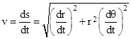
Expressed in modern (Leibnizian) notation, Newton’s solution began with the fact that, for any central force, the quantity h = r²(dθ/dt) is constant, where r and θ are the polar coordinates of the planet (the origin being at the center of the orbit). Also, since the line element in polar coordinates is

the speed v of the planet can be expressed in polar coordinates as

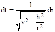
Substituting h/r² for dθ/dt in this expression, and then solving for dt, we get

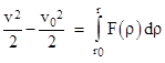
At this point, Newton invoked what we would regard as energy conservation, noting that the kinetic energy (per unit mass) of the planet is v²/2, and that the work done on the planet by the gravitational force equals the integral of Fdr, which is to say, the integral of the applied inward radial force F (which may be a function of r) over the radial distance traveled. Thus, letting v₀ denote the speed of the planet when it is at the radial position r₀, and letting v denote the speed of the planet after it has moved to some lower radial position r, we assert that the change in kinetic energy equals the work done by the gravitational force (which Newton had proven in Propositions 39 and 40), giving the relation

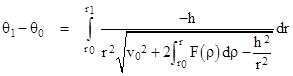
where F(r) is any given radial dependence of the gravitational force. Solving for v² and substituting into the previous equation, and integrating the left side, we get the integral relating times to the corresponding radial distances

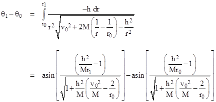
If we set F(r) = -M/r² , corresponding to an inverse square force law, it’s possible to evaluate this integral in closed form, giving an explicit equation for time as a function of radial position, but the integration is far from easy, and the resulting expression cannot be explicitly inverted to give a closed form expression for r as a function of t. However, to answer Halley’s question about the shape of the orbit, we really just need to determine the relation between r and θ, and we know that dθ = (h/r²)dt, so from the above equation we immediately have the corresponding equation relating the angular position to the radial position of the planet

For an inverse-square force (in units such that G = c = 1), we have F(r) = -M/r² where m is the mass of the central gravitating body (e.g., the sun), and so the integral appearing under the radical sign is

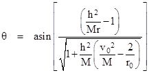
Inserting this into the previous equation and evaluating the main integral (which Newton assures us is “easy”), we get the result

Thus with a suitable choice of origin for the θ coordinate we have the relationship

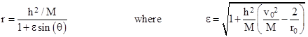
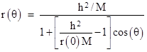
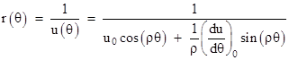
Solving this for r gives

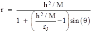
which is the equation of a conic (an ellipse if ε < 1) in polar coordinates with the origin at one focus. If we take the initial point r₀ to be the apogee or perigee, then v₀ = h/r₀, and the expression for the eccentricity simplifies, so the solution can be written as

In 1709 one of Newton’s followers, John Keill, published an analytical demonstration (using Newton’s fluctional notation, of course), making the argument more explicit than Newton had done, and perhaps thereby calling attention to the lack of substance in Newton’s argument. The following year, as Roger Cotes was beginning to edit the second edition of Principia, Newton sent him a few additional words to be added to the first corollary of Proposition 13. The entire demonstration then read as follows, with the words added in the second edition shown in italics:

From the three last Propositions it follows, that if any body P goes from the place P with any velocity in the direction of any right line PR, and at the same time is urged by the action of a centripetal force that is inversely proportional to the square of the distance of the places from the centre, the body will move in one of the conic sections, having its focus in the centre of force; and conversely. For the focus, the point of contact, and the position of the tangent, being given, a conic section may be described, which at that point shall have a given curvature. But the curvature is given from the centripetal force and velocity of the body being given; and two orbits, touching one the other, cannot be described by the same centripetal force [and the same velocity].

The final four words in brackets were actually not added until the third edition, published in 1726 just shortly before Newton’s death. This passage is usually called a “sketch of a proof”, but it seems slightly odd, if the proof was “very obvious” as Newton maintained, that he would present just a sketch of the proof, in contrast with the rather elaborately rigorous proofs given for such a multitude of other propositions. It’s also intriguing that he was so frugal with his words regarding this important proposition. Each edition contained just the most meager clarification, even though he knew full well that the passage was perceived to be unclear.

In 1710, prior to the appearance of the second edition of Principia, Johann Bernoulli published a critique of the first edition, pointing out that the first corollary to Proposition 13 had not been demonstrated, and that it certainly didn’t follow immediately from the converse proposition, as the first edition seemed to claim. Even after learning of the added words in the second edition, Bernoulli was unconvinced. To support his objection, Bernoulli noted that a similar sounding argument, when applied to inverse cube forces, would lead to a wrong conclusion. If a particle moves along any logarithmic spiral subject to a central force, it can be shown that the force varies as the reciprocal of the cube of the distance to the center, but the converse does not follow, because particles subject to an inverse cube force can follow other paths, such as hyperbolic spirals.

However, after the issue had been in dispute for nearly 10 years, Bernoulli ultimately (in 1720) acknowledged the legitimacy of Newton’s proof, and agreed that the inverse cube case was not a valid counter-example. Newton’s proof relies on the fact that the equations of motion involve only the second derivative of the particle’s position, so, given the initial position, direction, and speed of the particle (i.e., the zeroth and first derivatives), these equations can be uniquely integrated to give the path of a particle – a fact which is fairly intuitive because the equations explicitly give the second derivative of the particle’s position as a function of its position. (In later centuries, with increasing mathematical rigor, even this assertion would be considered to need a proof, but it was accepted as sufficiently obvious by all the participants in the controversy during Newton’s lifetime.) Furthermore, Newton had shown that all possible initial conditions can be achieved by a conic through a given point with a given focus – assuming an inverse square force. It follows (just as Newton said) that all possible solution paths for an inverse square force are conics. In contrast, a similar argument cannot be made for an inverse cube force and logarithmic spirals, because such spirals cannot produce all possible initial conditions. The other possible initial conditions correspond to the other species of paths that satisfy an inverse cube force.

Once this was explained, Bernoulli agreed that Newton’s proof was valid, although he continued to claim that the analytic approach using the Leibnizian notation was the surer way of achieving general and comprehensive results. Even though almost all modern scholars agree that Newton’s “sketch of a proof” was valid (at least in the third edition, and augmented with some fairly obvious supplemental statements),.modern science has followed Bernoulli’s advice, and no one today would dream of trying to approach such problems using the synthetic geometrical methods of Newton. In fact, Newton’s neo-classical methods were never used successfully by anyone other than himself. As the historian of science William Whewell wrote in 1847

The ponderous instrument of synthesis, so effective in his hands, has never since been grasped by one who could use it for such purposes; and we gaze at it with an admiring curiosity, as on some gigantic implement of war, which stands idle among the memorials of ancient days, and makes us wonder what manner of man he was who could wield as a weapon what we can hardly lift as a burden.

Surprisingly, though, the controversy over the validity of Newton’s key demonstrations has not entirely ended. To this day, there occasionally appear papers in scholarly journals complaining that Newton never actually gave a valid answer to Halley’s question, and specifically that the reasoning presented in support of Corollary 1 of Proposition 13, even in the third edition, is inadequate if not outright specious. Such charges are invariably met with a flurry of responses, carefully explaining the subtle force of Newton’s reasoning, and disposing of purported counter-examples.

Adding to the confusion of these discussions, Newton once seemed to imply that Proposition 17 gives a rigorous answer to Halley’s original question. This proposition does indeed give explicit constructions for the path of a planet subjected to a central inverse-square force, but the demonstration explicitly assumes that the path is a conic. Unfortunately, this stipulation is not mentioned in the statement of the proposition itself, so the content of the proposition has sometimes been misconstrued. It gives the elliptical, parabolic, or hyperbolic paths explicitly for a given set of initial conditions, but only on the assumption that the path is a conic, which is why Corollary 1 to Proposition 13 is needed, to establish that the path must be a conic. This again emphasizes the importance of the corollary, the very answer to Halley’s original question, making it all the more odd that Newton was so persistently reticent about it’s explicit demonstration. Perhaps he was conscious of the need for an explicit use of calculus to do justice to the demonstration, and he had been unwilling (at least in the first edition) to reveal many of the techniques he possessed.

Today the derivation of Kepler’s first law is a simple exercise, but there is an interesting variety of popular methods, invoking such things as complex numbers, vector analysis, reciprocal substitutions, and so on. Perhaps the most straightforward approach is to differentiate rectilinear coordinates x = r cos(θ) and y = r sin(θ) twice with respect to time, and then set the radial component of acceleration to the negative of the central force, and the tangential component to zero, giving the equations

The right hand equation is equivalent to d(r²ω)/dt = 0, and hence the quantity h = r²ω is a constant. Letting u denote the reciprocal of r, we have r = u^-1 and h/ω = u^-2, from which it follows that

where we have used the fact that ω = dθ/dt. Substituting for ω and r in the radial equation of motion, we get

Simplifying, we arrive at the familiar equation for the path of a test particle in a stationary spherical gravitational field according to Newtonian theory

The general solution can be expressed as the sum of the particular solution u_p = M/h² and the solution of the homogeneous equation. The latter can be expressed in terms of the characteristic values ±i as

where A and B are constants determined by the initial conditions, for which we can take the zeroth and first derivatives of u(θ) = u_H+ u_p at θ = 0. Thus we have the conditions

A persistent orbit must have points at which du/dθ = 0, and we can place the zero of our angular coordinate at such a point, in which case the right hand condition implies A = B, and hence the left hand condition gives A = B = [u(0) – m/h²]/2. Therefore the general solution of the equation of motion (for an inverse square force) is

Reverting back to the radial equation, the gives

which is seen to be identical to the previous result as derived by following Newton’s method, since we can shift the origin of the angular coordinate by π/2 to convert the cosine to sine.

It’s interesting to examine why an inverse cube force law leads to such different families of paths. (Roger Cotes wrote a paper on this subject in 1714, identifying the five distinct species of solutions, thereby clarifying the significance of Bernoulli’s objection. This analysis was included in Cotes’s book Harmonia Mensurarum.) Following the same approach as above, but replacing the force –m/r² with the inverse cube force –M/r³, we arrive at the differential equation

in terms of the reciprocal parameter u = 1/r. What had been a constant term M/h² on the right hand side in the case of an inverse square law is now multiplied by u, due to the extra factor of r in the denominator of the force term, so it is brought over to the left side. One might think this would lead to an even simpler solution, since the equation in this case is homogeneous. However, the coefficient of u in this homogeneous equation is now dependent on the ratio of M to h², and can be positive, negative, or zero. As a result, there are multiple cases to consider, in contrast with the differential equation based on an inverse square force, for which the homogeneous equation has constant coefficients of unity. Thus, for the inverse square force, the characteristic values were simply ±i, whereas for the inverse cube force the characteristic values are ±λ where

which may be real, imaginary, or zero accordingly as M is greater than, less than, or equal to h². If M equals h² the differential equation reduces to d²u/dθ² = 0, which has the general solution u = Aθ + B for constants A and B. If A = 0, then u and r are constant, signifying that the path is a circle. If A is not zero, then with a suitable choice of angular origin the path can be expressed as a hyperbolic spiral

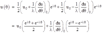
for some constant k. If m does not equal h², we have two unequal characteristic roots ±λ, and the general form of the solution is

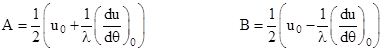
for some constants A and B, which are determined by the initial conditions, e.g., by the zeroth and first derivatives of u with respect to θ at the initial angle θ = 0. Letting u₀ and (du/dθ)₀ denote these initial conditions, we have

Therefore the constants are

If u₀ happens to equal (1/λ)(du/dθ)₀, which of course can only be the case if λ is real, then one of these coefficients is zero, and the solution is a simple logarithmic spiral, i.e., it can be written in the form

for real constants R and k. On the other hand, if neither A nor B vanishes, but A = ±B, then the solution is

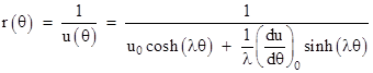
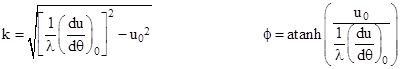
If λ is real, these can be written in terms of hyperbolic trigonometric functions as

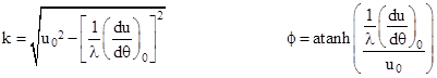
respectively. If λ is imaginary, we have a real value r such that λ = iρ, and we can express the solution in terms of the ordinary trigonometric functions as

Of course, the sine function can be converted to a cosine function by a simple shift of the zero point of the angular coordinate, so both of these represent the same class of orbital shapes. The same is not true of the hyperbolic functions, because cosh and sinh cannot be transformed into each other by a shift of the argument.

If A and B have distinct non-zero magnitudes, then the solution for u(θ) can be written in the form

Again, if λ is real, we can use the hyperbolic trigonometric functions to express the solution as

If λ is imaginary, we have a real value ρ such that λ = iρ, and we can express the solution in terms of the ordinary trigonometric functions as

These might seem to represent an increased class of solutions, but in fact they do not give any shapes beyond those in the solutions described previously. To see why, we first observe that for either of these last two solutions, if the path contains a perigee, i.e., a local minimum where dr/dθ = 0, then we can choose that point as θ = 0, and the second terms in the denominators vanish, so the solutions can be written as

respectively. This leaves only the paths that do not contain any local minimum, i.e., monotonically increasing or decreasing spirals. However, even in these cases the above equations reduce to the formed described previously. To see why, suppose the magnitude of u₀ is less than the magnitude of (1/λ)(du/dθ)₀. In that case we can define the real values

so we have

Hence the solution can be written as

Similarly, if the magnitude of u₀ is greater than the magnitude of (1/λ)(du/dθ)₀, we can define the real values

so we have

Hence the solution can be written as

Thus the complete set of possible shapes for the path of a planet moving in an inverse square force field consists of the five “species” of spirals (as identified by Roger Cotes in 1714)

Admittedly this classification into “species” is somewhat arbitrary, but it does serve to highlight the variety of possible cases for an inverse cube force in comparison with the conic sections for an inverse square force. Incidentally, modern courses in celestial mechanics often answer Halley’s original question by giving a demonstration in terms of vector analysis, beginning with the basic inverse square equation of motion

If we cross multiply both sides by r, and recall that r x r is identically zero, we see that

Making use of this fact, and the chain rule for differentiation, we have

from which we infer that the vector

is constant. This vector is perpendicular to the plane containing the sun, the planet, and the velocity vector of the planet, so it follows that the planet always remains in a single plane of motion. Now, suppose we cross multiply the original equation of motion by this constant vector h. Recalling that the sign of a cross product is reversed under commutation, we get

By the vector triple product identity (a x b) x c = (a∙c)b – (b∙c)a, we can expand the triple product on the right side, leading to the equation

Recall that r∙r = r², and if we differentiate both sides of that relation we get . Therefore, the above equation can be written as

Now we observe that the left side is a simple derivative, i.e.,

where we’ve made use of the fact that dh/dt = 0. Also, the cross product on the right hand side of the prior equation can be written as a simple derivative, as shown by

Substituting these derivatives into the prior equation, we get

Integrating both sides, this leads to

where the vector C is the constant of integration. Finally, to reduce this to a scalar equation, we take the dot product of both sides with r, which gives

Making use of the vector identity a ∙ b x c = a x b ∙ c on the left hand side, recalling that , and letting θ denote the angle between the vectors r and C, this equation reduces to

Solving this for r gives the equation of a conic

This gives an explicit answer to Halley’s original question, and although it seems somewhat elaborate, it is considerably more succinct than the seven pages of calculus it took Bernoulli to present his derivation in 1710. This vector derivation is comparable in length to the scalar component derivation given previously, but it seems to involve steps that are not particularly intuitive. It gives the impression of having been constructed by working backwards from the answer. Also, it is purely ad hoc for the inverse square case; no similar demonstration exists for other cases, such as an inverse cube force. The scalar component derivation leading to an ordinary linear differential equation is perhaps more straightforward, and certainly quite general, but it relies on the reciprocal radius substitution, which is not an obvious step. All things considered, the most natural and intuitive demonstration seems to be Newton’s.

Incidentally, notice that Newton’s Proposition 41, expressed analytically by equation (1) can also be differentiated and written in the form

where we have set F(r) = M/r² to represent an inverse-square force of gravitation. Differentiating this again and dividing through by 2(dr/dt), we have

Thus Newton’s Proposition 41 for an inverse square centripetal force implies that the radial parameter r satisfies this second-order differential equation. Of course, in order to solve this equation we must integrate it twice, bringing us back to the form in which Newton presented it. Nevertheless, the differential form is interesting. Leibniz was among the first to translate the results of Newton’s Principia into analytic form, and to express the governing conditions on a physical process explicitly as a differential equation. Noting that h = r²ω, the above equation is the same as the left hand equation (2), which shows that the second term on the right side of the above equation is a component of the absolute acceleration, although it can also be regarded as a fictitious centrifugal force.

Return to MathPages Main Menu