Galileo’s Catenary

Near the end of Day Four of “Dialogues Concerning Two New Sciences” (1638), Galileo discusses the parabolic shape of ballistic trajectories (assuming constant gravity and no wind resistance), and makes the following observation

I must tell you something which will both surprise and please you, namely, that a cord stretched more or less tightly assumes a curve which closely approximates a parabola. This similarity is clearly seen if you draw a parabolic curve on a vertical plane and then invert it so that the apex will lie at the bottom and the base remain horizontal; for, on hanging a chain below the base, one end attached to each extremity of the base, you will observe that, on slackening the chain more or less, it bends and fits itself to the parabola; and the coincidence is more exact in proportion as the parabola is drawn with less curvature or, so to speak, more stretched; so that using parabolas described with elevations less than 45° the chain fits its parabola almost perfectly.

He immediately goes on to say “Then with a fine chain one would be able to quickly draw many parabolic lines upon a plane surface”, which is significant because it echoes the statement made on Day Two that a chain can be used to draw parabolas. Based on that statement from Day Two, many historians have reported that Galileo claimed the curve of a hanging chain is exactly parabolic. But we can see from the appearance of the same remark on Day Four that it clearly refers to an approximate correspondence, good enough for practical purposes (such as artillery calculations, or tapering a beam by an “ordinary mechanic” as discussed on Day Two) for sufficiently shallow curves.

After Galileo’s death, one of his assistants, Vincenzo Viviani, wrote some comments about Galileo’s plans for Day Five of the Dialogues (which Galileo was unable to complete), in which (according to Viviani) Galileo intended to present a proof that the hanging chain curve was exactly parabolic. I believe this was a misunderstanding on the part of Viviani, and that Galileo was actually thinking of a demonstration that the so-called catenary (from the Latin catena for chain) approaches arbitrarily close to a parabola as it becomes flatter, as he explicitly says on Day Four. His purpose was to use the chain as a kind of primitive analog computer to represent parabolic trajectories (for artillery), at least those with an original angle less than 45° up from horizontal. Interestingly, his conviction that the two curves were asymptotically the same apparently came from his observation that it is impossible to pull a cord perfectly horizontal, and he associated this with the fact that the path of a ballistic projectile cannot be perfectly horizontal. In the one case it would take infinite tension in the cable, and in the other case it would take infinite velocity of the projectile. Somehow from this he intuited that the curves must be asymptotically the same.

From one point of view the close approximation of the catenary to a parabola is trivial, since (for equal heights of the end points) the curve is obviously symmetrical and therefore “even” ordered, so if we translate the center of the curve at the origin of Cartesian coordinates the lowest order term is proportional to x², i.e., parabolic. However, the closeness of the curves is actually stronger than this would suggest. It’s slightly non-trivial to explain why the catenary with 45° at the end point is as close to a parabolic shape as it is.

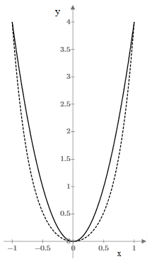
It’s clear that Galileo had empirically compared chains with parabolas, so he couldn’t have failed to see that they are not generally the same. For example, consider the parabola and catenary shown superimposed below.

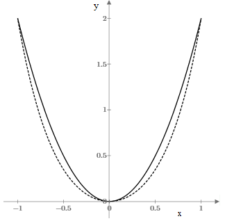
The solid curve is a parabola y = 4x² tangent to the x axis, and the dashed curve is the catenary with matched points at x = ±1. Even for the somewhat less steep curve y = 2x² the corresponding catenary is still obviously different, as shown below.

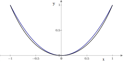
The curves begin to appear more similar when we consider the parabola y = x² and the corresponding catenary, as shown below.

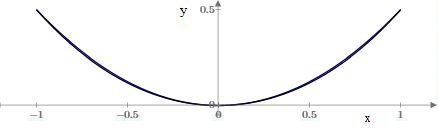
Still, at this level the curves remain noticeably distinct. Galileo’s observation that the curves were very similar referred to cases for which the slope at the end points is less than 45°, which corresponds to the parabola y = (1/2)x². Indeed, as shown in the figure below, the curves are visually almost indistinguishable in this case.

For shallower curves the fit is even better. Galileo found this first by experiment, and his objective was to prove that the catenary is indeed asymptotically parabolic. As discussed above, this is obviously true for any “even” curve with sufficient shallowness, but he wanted to show that the curves are closely asymptotic even for slopes as great as 45°. He apparently had in mind a plausibility argument based on the fact that a cable that is loaded uniformly as a function of x (such as the cables of a suspension bridge) has a parabolic shape, and the loading of a cable just under its own weight approaches uniformity as the cable approaches straightness. However, as shown in the figure above, the catenary is quite close to a parabola even with significant curvature. Galileo also considered a solid horizontal beam supported at the ends, and found the “total moment” due to a force applied at some intermediate point to be proportional to the product of the distances from that point to the ends, which gives a parabolic function, but how this is related to the positions of the parts of a chain is unclear. He never completed Day Five of the dialogues, so we can only guess what he had in mind.

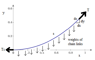
To assess how closely the catenary approaches a parabolic shape, we will first derive its exact idealized equation. The original approach taken by John Bernoulli in 1691 was to consider the portion of the chain of length s extending from the central point to some arbitrary distance as a body in equilibrium subject to forces in three directions, namely, the tensions T₀ and T at the ends of this segment and the downward weights along the segment, as shown below.

The weight per unit length along the chain is constant, but the weight per unit of horizontal distance x is not constant, because of the changing slope of the chain. However, Bernoulli realized that the sums of the forces in the vertical and horizontal directions must vanish, regardless of how they are distributed (since we know the moments are balanced). Hence the weights can be represented by the single downward force W = ρs applied to this segment, where ρ is the weight density of the chain per unit length. Thus we have

from which we immediately get

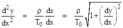
Differentiating with respect to x gives

Thus in terms of the variable u = dy/dx we have

This was Bernoulli’s result, expressing x as a transcendental integral of a function of u = dy/dx. Today we recognize the integral of the left side as the inverse hyperbolic sine, so we can write dy/dx = sinh(x/A) where A = T₀/ρ. Integrating this and choosing the constant of integration to place the center of the curve at the origin gives the familiar expression y = cosh(x/A) – A.

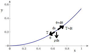
This is a nice derivation, but it relies on the slightly non-trivial physical reasoning about combining the distributed weights without regard to moments, and also on knowledge of the integral and the modern understanding of the hyperbolic functions. For a less succinct but perhaps more complete and self-contained approach focusing on just a single incremental segment ds, let T denote the tension in the cable at the beginning of that segment, θ the angle that the cable makes with horizontal at that point, and s the path length parameter along the cable (measured from the centeral point). This is depicted in the figure below.

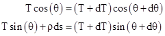
A balance of horizontal and vertical forces (respectively) on the incremental segment ds of the cable gives

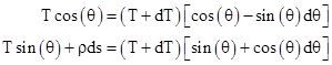
Making use of the trigonometric identities cos(a+b) = cos(a)cos(b) + sin(a)sin(b) and sin(a+b) = sin(a)cos(b) + cos(a)sin(b), and the fact that as x approaches zero the value of cos(x) goes to 1 and the value of sin(x) goes to x, these equations reduce to

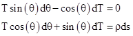
Dropping the products of differentials and simplifying, we get

Multiplying through the first by sin(θ) and the second by cos(θ) and adding the two equations together, we get

Also, the first of the previous two equations gives

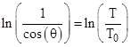
which can be integrated to give

where T₀ is a constant of integration equal to the tension at the central point of the cable at which θ = 0. Taking the exponential of both sides, we have

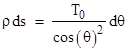
Substituting for T in (1) gives

Integrating this from s=0 at the center, we get the relation

Noting that tan(θ) = dy/dx, we have

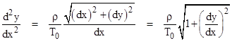
Also, since (ds)² = (dx)² + (dy)², we can write

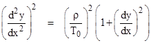
At this point we could put u = dy/dx and integrate (ρ/T₀)dx = du/√(1+u²), assuming we know that this integral is the hyperbolic sine, but another approach is to square both sides to give

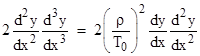
Differentiating again with respect to x gives

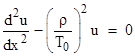
Dividing through by 2(d²y/dx²), and putting u = dy/dx, we get the second order differential equation

The two distinct roots of the characteristic polynomial are ±ρ/T₀, so the general form of the solution is

Since u = dy/dx = 0 at x=0 we have A₁ = −A₂, and by taking the derivative with respect to x and making use of (2), noting that ds/dx = 1 at x=0, we have A₁ = −A₂ = 1/2, and hence (defining the hyperbolic function, instead of smuggling it)

Integrating this we arrive at the result

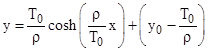
To place the curve tangent to the x axis at the origin, we set y₀ = 0, and for any constant A = T₀/ρ the general catenary equation can be written in the form

Expanding this into a series, we have

As noted above, for sufficiently small x/A this obviously approaches a parabolic shape, since the lowest-order term is the squared term. Compared with the parabola given by x²/(2A), which is also tangent to the x axis at the origin, the maximum deviation over the range from x = 0 to 1 occurs at the end point (x=1), where the curves differ by 1/(24A³), neglecting the higher order terms. The 45° case corresponds to A=1, so the deviation is 1/24 of the half-span. However, the actual comparison should be with a parabola that coincides with the catenary at the central point and the end points. In other words, we want the parabola x = x²/(2B) where B is defined such that the parabola equals the catenary at the end points (x = ±1), so we choose B such that

Hence, focusing on just the first two terms, the equations of the catenary and corresponding parabola are

and the difference between them is x²(1−x²)/(24A³), which equals zero at x = 0 and 1, and reaches a maximum at x = 1/√2. Consequently, the maximum deviation is 1/(96A³), which is only about 1% of the half-span in the 45° case (i.e., the case A=1). For shallower cases, the value of A is greater than 1, so the factor of A³ in the denominator causes further reduction in the maximum deviation.

The catenary is also the shape that minimizes the potential energy of a chain of a given length between two points (and, equivalently, that minimizes the length for a given potential energy), as can be derived using the calculus of variations. The potential energy (assuming constant acceleration of gravity) is just the integral of yds, and since (ds)² = (dx)² + (dy)², we want the function y(x) that minimizes the integral of  where dots signify derivatives with respect to x, and

The Euler-Lagrange equation provides the condition that must be satisfied in order for the integral to be “stationary” (which is usually an extremal condition), namely

Carrying out the differentiations and simplifying, this gives the condition

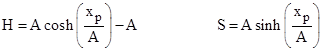
which has the solution y = A cosh(x/A) for an arbitrary constant A. Notice that we did not impose any length constraint in this derivation because we can obviously shift the zero point of y and adjust the constant A to give any achievable length. (It is traditional in the literature to present the derivation with the length constraint, but that simply replaces y with y−λ for some constant λ, which is nothing but a shift in the zero point of y.)

It can also be shown that the catenary is the path swept out by the focus of a parabola rolling on a flat line.

As an aside, one modern corporation supposedly asked a question about a hanging chain in its job interviews. The question posited a chain of length 80 feet hanging between the tops of two posts, each 50 feet tall, and the center of the chain is 10 feet above the ground. How far apart are the posts? Obviously the vertical distance of each half-span is 40 feet, for a total vertical travel of 80 feet, which is the length of the chain, so there can be no horizontal component at all, and hence the posts must have no distance between them, i.e., the chain is hanging vertically, dropping straight down and rising straight back up. Thus the question is degenerate (perhaps intended to weed out applicants who think from the general to the particular?), but with different parameters it provides an interesting application of the catenary formula noted above.

In general, suppose the center of the chain is a vertical distance H below the top of the posts, and let x_p denote the distance from the center line to one post, and let S denote half the length of the cable, i.e., the length from the center point to one end. (In our example, the whole cable is 80 feet long, so S=40 feet.) Making use of equations (2), (3) and (4), and recalling that A = T₀/ρ, we have

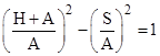
(This is formally identical to the parametric equations for hyperbolic motion discussed Accelerated Travels, with x_p, H, S, and A corresponding to τ, x, t, and a₀ respectively.) Solving these for cosh and sinh and substituting into the identity cosh(z)² – sinh(z)² = 1, we have

Solving this for the parameter A gives

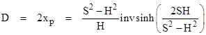
Inserting this value into the expression for S and solving for x_p, we get the distance D between the two posts

Naturally this approaches 2S as H goes to 0, and it approaches 0 as H goes to S (as in the interview question).

Return to MathPages Main Menu