The Arsenal Companion

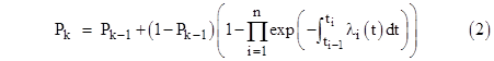
Appendix 3 of the ‘Arsenal’ draft Advisory Circular (AC) 25.1309 defines the normalized average probability (also called “Average Probability per Flight Hour”) of a failure condition as

where N is the number of flights in the life of a single airplane, T_F is the duration of each flight, and P_k is the probability of the failure condition on the kth flight.  For a failure condition consisting of a single element on a flight with n phases, the probability P_k is given recursively (between detection/repairs) by

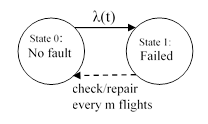
where P_k−1 is the “prior” probability, i.e., the probability that the element is already failed at the start of the certain flight, and λ_i(t) is the hazard rate function for the ith phase extending from t_i−1 to t_i.  (For the derivation of this formula, see the note on Hazard Rate Function.)  If the element is checked and repaired before the certain flight, then P_k−1 is set to zero, which implies that the probability of the failed state at the end of the previous flight is transferred to the un-failed state. For a system that is checked and repaired every m flights, the 2-state Markov model for a single flight in this simple case can be depicted as shown below.

where λ(t) denotes the piecewise aggregate failure rate functions for the n phases of the flight. It can be shown (see Note 5 in Normalized Average Probability) that the argument of the exponential function in equation (2) is simply –λ_meanT_F if we define λ_mean as the mean failure rate of the element during a flight, so equation (2) can be written as

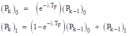
Hereafter we will drop the “mean” suffix from λ_mean and simply refer to the mean failure rate for a flight as λ. Letting (P_k)₀ and (P_k)₁ denote the probabilities of the healthy and failed states respectively for the kth flight, and recalling that (P_k)₀ + (P_k)₁ = 1, this equation is equivalent to the pair of relations

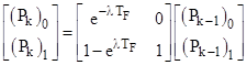
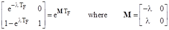
In matrix form these equations can be written as

The coefficient matrix is given in terms of the mean failure rate matrix M by

So, letting P_k denote the state vector [(P_k)₀, (P_k)₁]^T, equation (2) can be written as

which is simply the solution of the homogeneous state equation dP/dt = MP. This equation applies provided no inspection/repairs occur between the end of the (k−1)th flight and the beginning of the kth flight. If the element is checked and repaired prior to a certain flight, we replace the prior state vector with [1, 0]^T.  More generally, if the element is checked and repaired prior to the mth flight, we replace the prior state vector with [1,0]^T whenever k−1 is a multiple of m. In matrix form, this reset is accomplished by multiplying the state vector at the end of the (k−1)th flight by

where α = 0 if k−1 is a multiple of m, and otherwise α = 1. Therefore, taking the periodic repairs into account, the probability of the failure condition for the kth flight is given recursively by

This covers both active and latent failures. For an element that is checked and repaired prior to each flight, we set m=1, meaning the state vector is reset prior to each flight. Writing the state equations in matrix form makes it immediately apparent how they apply unchanged to failure combinations of any number of elements (not just a single element), and how they account for any specified periodic inspection/repair intervals.  It also accounts for any “required order” effects. An example for a failure combination of three components is shown in another article.

Ordinarily one would proceed from the basic state equation and its solution (5) to show that it reduces to equation (2) for a single element with no repair presented in the Arsenal, but in the preceding discussion we worked in the opposite direction, to show by “reverse engineering” that the calculation specified in the Arsenal AC implies the general method. This has sometimes been disputed, both in the industry and within the regulatory agencies.

One area of disagreement has been the treatment of latent failure conditions. This subject has led to contradictory statements by the regulatory agencies, who have sometimes stated that latent failure conditions cannot be assigned hazard levels at all, and at other times have stated that latent failure conditions that leave the airplane a single fault away from jeopardizing safe operation must be treated as Hazardous and shown to be extremely remote.

To clear up the confusion, some historical background is useful. Numerical probability analysis methods for airworthiness certification were originally applied mainly to catastrophic or hazardous failure conditions involving obvious effects, and it’s clear that the probability of a catastrophic failure condition arising on a given flight is the same as the probability of it being present during that flight. However, some recent regulatory guidance for 25.901(c), known as “latent plus one”, imposes quantitative probability requirements on totally latent failure conditions that are one failure away from a catastrophic condition. The probability of a latent failure condition arising on a given flight is very different from the probability of it being present on that flight... indeed, the unique risk posed by latent failure conditions is precisely their continued presence on flights after the flight on which they first arise. A meaningful assessment of the risk associated with a latent failure condition must account, not just for the expected number of flights during which the condition arises, but for the expected number of flights during which the condition is present, because this represents the exposure to a subsequent fault that results in a catastrophic condition.

As explained above, the numerical probability criteria described in the referenced Arsenal AC 25.1309 account for the difference between active and latent faults by explicitly specifying that if the state of a failure condition is unknown at the beginning of a certain flight, then the probability of the condition during that flight equals the probability of the condition arising on that flight plus the probability that the condition is already present at the beginning of the flight (having arisen on a previous flight and not been repaired). Thus, the FAA requirement for the latent failure (combination) to be extremely remote per the Arsenal AC terminology means that the normalized average probability as computed above must be on the order of 1E-07/FH or less.

In the simple case of a single element with a latent exposure time to T_L and constant failure rate λ, the Arsenal calculation gives the normalized average probability (for rare events) of approximately [(1/2)/T_F](λT_L).  The factor is square brackets represents the averaging and normalization. If the requirement was for this latent failure condition to be remote (rather than extremely remote) per the Arsenal definition, then for a fleet with average flight length T_F = 5 hours the requirement would be λT_L < 1E-04.  This would be just slightly more restrictive than the EASA requirement, and the proposed future FAA requirements (judging from draft NPRM materials) for dealing with latent fault, which impose a “1/1000” requirement defined as λT_L < 1E-03.  However, the actual “latent plus one” requirement promulgated by the FAA for 25.901(c) calls for the latent part to be extremely remote (even though the preamble to which the FAA refers as the source of this requirement specified that the latent parts must be “not foreseeable”, which they define in this context is extremely improbable), meaning in this example it requires λT_L < 1E-06, so it is three orders of magnitude more stringent than the corresponding EASA and proposed future FAA requirements.

As an aside, the FAA has frequently asserted that, for a single latent element, the normalized average probability (as defined in the Arsenal) equals the failure rate λ, independent of the latency period. That would be a correct statement if they were referring to active faults, but it is plainly incorrect for latent faults, as discussed above, and as easily confirmed by applying the Arsenal calculation to this case.  (It’s also clearly inconsistent with the fact that a meaningful limit on the risk of a latent fault must involve the product λT_L as in the Arsenal and EASA and proposed future FAA requirements.)  Underlying this mistake are three inter-related misunderstandings:  First is the idea that we need not account for the fact that latent faults can persist for multiple flight. This misleads people into thinking that the relevant probability for a latent fault condition is the probability of the transition, which is obviously senseless. Second, there is a misunderstanding of the meaning and purpose of normalization (see article). Third is the failure to distinguish between active failure conditions consisting of individually latent failures versus actual latent failure conditions, to which we now turn.

Consider a case of three individually latent components, and suppose that if all three of those components are failed, a catastrophic event may occur.  This is obviously not a latent failure condition, even though the three elements are individually latent.  Having any one or two of them failed is a latent condition, but the third one to fail is not latent (under the stated assumptions).  This is the kind of situation that is treated in sample calculations in ARP 4761. In such cases, the overall failure condition obviously cannot be carried over from a prior flight, so, in effect, the calculation includes a per-flight check/repair of the overall failure condition, and the relevant probability is the probability of transitioning into the fully-failed state during a flight.

However, this is not a latent failure condition, even though it consists entirely of individually latent failures.  To perform a “latent plus one” calculation on such a system (in addition to showing that the overall condition of all three elements being failed meets 1E-09), we need to show that any combination of two of those failures (which leave us one failure away from a catastrophic condition) are extremely remote.  Those two-failure combinations are genuinely latent, and can persist for multiple flights, so they must be treated per the Arsenal calculation for latent failures. 

For control system failures involving loss of two parallel alert lights and the loss of (say) overspeed protection, this entire combination of three faults is totally latent, and can persist for many flights.  Indeed this is the entire problem posed by the latency, i.e., it allows dispatch in a non-dispatchable condition.  Therefore, the relevant probability is the probability of this condition being present on a given flight, not the probability that it arises on that flight. This is a valid measure of the risk posed by this truly latent failure condition.

The Arsenal AC cites examples of probability calculations in ARP 4761, but the cited examples don’t actually discuss latent failure conditions, they discuss active failure conditions with latent components. Much of the confusion in this area is due to people attempting to apply the formulas for active combinations of latent failures to truly latent combinations of failures.  (In one example the ARP does correctly compute the average per-flight probability of a genuinely latent failure condition, but then erroneously applies a spurious factor that is tantamount to assuming the system is checked and repaired before each flight.) The genuinely applicable guidance in ARP 4761 for all kinds of systems is the generic modeling techniques described in the section on Markov models.  Note that the draft update, ARP 4761A, has an enhanced version of the Markov model section.  Those discussions are correct, and consistent with the Arsenal calculation method described above.

Return to MathPages Main Menu