Failure Rates and Normalized Probabilities

Section D.11.1.5 of ARP 4761 presents examples of reliability calculations for various combinations of active and latent faults. Two sections of particular interest are D.11.1.5.3 and D.11.1.5.5, both of which have sometimes been cited as examples of calculations for completely latent failure conditions. However, the example in D.11.5.3 is not actually a latent failure condition, because although it applies to a system in which each of the two elements can individually fail latently, the failure of both elements results in an obvious loss of function, leading to detection and repair before the next flight. Hence “at least one of the items must be operating at the start of each flight”. For such a system, the probability of a failure condition arising on a given flight is equal to the probability of it occurring (i.e., being present, see Note 1) on that flight.

The end of section D.11.5.3 says the “average probability calculation” for this example is described in section D.11.1.5.5, thereby linking the two examples together, and yet the latter section discusses a genuinely latent failure condition. Obviously the risk for a failure condition isn’t independent of whether or not the condition is checked and repaired before each flight. (If it were, the regulatory agencies wouldn’t care if the condition was latent or not.)  The two ostensibly different examples in the ARP give the same “result” because D.11.1.5.5 does not present a calculation of the normalized average probability (as called for by the Arsenal AC 25.1309), it presents an approximate calculation of the average rate for the failure condition. It is certainly possible to use the elementary aspects of probability theory described in the ARP to compute the normalized average probability, but this isn’t what section D.11.1.5.5 is calculating. The quantity computed in this section has the same value, regardless of whether or not a per-flight check and repair is performed on the failure condition, meaning this quantity is not a meaningful measure of the risk due to the latent failure condition.

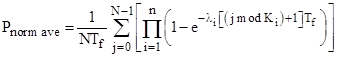
To show this, recall that the system discussed in section D.11.1.5.5 consists of two independent components C₁ and C₂ with constant failure rates λ₁ and λ₂ and latency periods T₁ and T₂ = k T₁ respectively, where k is a positive integer and T_f is the average flight duration. Note that the ARP is confining itself to the special case where T₂ is a multiple of T₁, but this restrictions is not necessary. As shown in the article on Probability for Regulatory Requirements, for a cutset with n components with constant failure rates λ₁, λ₂, …, λ_n and completely independent inspection/repair intervals K₁, K₂, …, K_n flights, the normalized average probability (also called “Average Probability per Flight Hour”) as defined by the Arsenal AC 25.1309 is given simply by

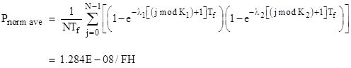
where N is the least common multiple of the K_i values. (We can also set N to the number of flights in the life of an airplane.) For concreteness, consider the case with λ₁ = 1.5E-06/hr, λ₂ = 1.2E-07/hr, T_f=5 hr, T₁ = 500 hr, T₂ = 2500 hr. The number of flights in the T₁ interval is K₁ = 100, and the number of flights in the T₂ interval is K₂ = 500. We set N equal to the least common multiple, so N=500. So, in this case the normalized average probability of this failure condition is

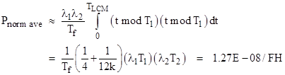
If the flight duration is small compared with the latency periods, and if the probabilities are all orders of magnitude smaller than 1, this can be approximated (as explained in Average Product of Sawtooth Functions) by the integral

where k = T₂/T₁. This is slightly less than the exact value given previously, because it is based on the continuous average, whereas the exact value is based on the average of the discrete values at the end of each flight.  This approach immediately generalizes to cutsets with three or more components.

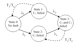
However, if the inspection/repair intervals for the components are not independent, these simple formulas can’t be used. For example, we may have two components that are individually completely latent, so each could be failed for the life of the airplane, but if they are both failed, this condition may be checked and repaired at some specified interval. For such a system, the above equations are not applicable, and we must account for the repair transitions that are applied to combined states. This can be accomplished using a Markov model. For example, the system described in the example from section D.11.1.5.5 corresponds to the Markov model depicted below

The dashed transition signify that the probability of the source state is moved to the destination state every T₁/T_f flights. We haven’t shown the discrete repair transitions at the T₂ interval because we will run the model only up to the least common multiple of T₁ and T₂, which in the restricted case of the ARP example is just T₂. The exact solution, following the Arsenal AC definition (see The Arsenal Companion and Latencies and Periodic Repairs), is

where N is the number of missions in the life of the vehicle (or, equivalently, the least common multiple of the latency intervals), and P_j is the probability state vector at the end of the jth flight, given recursively by

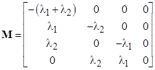
Here M is the mean failure rate matrix, which in our example is

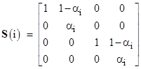
The inspection/repair transition matrix S(j−1) between the end of the (j−1)th flight and the beginning of the jth flight is given by

where α_i = 0 if i is divisible by T₁/T_F and otherwise α_i = 1. For the specific numerical example discussed above, this gives the result

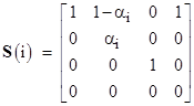
in agreement with the exact result given previously. Now, before we review the ARP calculation, suppose we implement a per-flight check and repair of State 3, i.e., the fully failed state. The calculation is exactly as above, except that the S matrix is

This gives the result

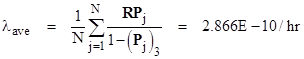
The corresponds to the case in section D.11.1.5.3, which is not actual a latent failure condition, as discussed above, because it assume the fully latently failed state is detected and repaired prior to each flight. On the other hand, instead of computing the normalized average probability of the failure condition, suppose we are interested in the average rate at which the system enters State 3. That rate is given by [λ₂(P)₁ + λ₁(P)₂]/(1−(P)₃), so the Markov solution gives

where R = [0, λ₂, λ₁, 0]. This is essentially equal numerically to the normalized average probability for the case where we detect and repair the fully-failed state before every flight. In the rare event approximation these are essentially the same thing, because in both cases we are just computing the probability of entering state 3 during a given flight, rather than the probability of being in state 3 at some point during the flight. This corresponds to the two different meanings of the word “occur” (see Note 1), and the Arsenal AC 25.1309 unambiguously defines the normalized average probability in terms of the probability of the failure condition being present during a flight… which is a meaningful measure of the risk associated with latent faults. This is consistent with the historical treatment of latent faults, and is also confirmed by the EASA Amendment 24 and the FAA NPRM proposals to quantify the risk of latent faults in terms of the product of the failure rate and the exposure time.

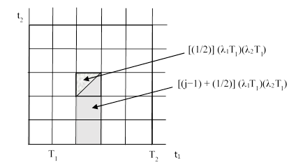
With the above background, we can examine the example in section D.11.1.5.5 of ARP 4761. In the rare event approximation, letting t₁ and t₂ denote the times at which components C₁ and C₂ fail, the probability of entering the fully-failed state during the jth T₁ interval can be read directly from the diagram below.

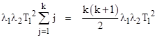
Thus the approximate probability of entering the fully failed state during the jth T₁ interval is jλ₁λ₂T₁², so the probability of entering the fully-failed state during the entire T₂ interval (which consists of k intervals of duration T₁) is

It should be noted that this not the probability of the failure condition at the end of the T₂ interval, since that probability is reset k times, and is a sawtooth function because of the detect/repair transition every T₁ hours. The above quantity represents just the cumulative flow into the fully-failed state during the T₂ interval. Dividing this by T₂ gives the approximate average failure rate

The ARP actually multiplies the above quantity by the average flight length, to give the average probability of entering the failure condition for a flight (not the probability of the failure condition on that flight), and then divides by the average flight length to give the rate per hour. As expected, this is the same as the average failure rate computing using the general Markov model method, which is numerically equal to the normalized average probability for the case where the fully-failed state is checked and repaired prior to each flight. In contrast, the normalized average probability for the fully latent failure condition is 1.284E-08/FH, as computed by direct calculation and by the Markov model previously.

As can be seen from the above discussion, neither section D.11.1.5.3 nor section D.11.1.5.5 of ARP 4761 provides a calculation of the normalized average probability of a fully latent failure condition as defined in Appendix 3 of the draft Arsenal AC 25.1309. The former section doesn’t address a latent failure condition at all, and the latter section computes (for a very restricted case that does not generalize) an approximation of the average failure rate, which would equal the normalized average probability only if the failure condition was checked and repaired prior to each flight, which is not the case for a genuinely latent failure condition. Of course, making use of the elementary probability theory discussed in ARP 4761, and particularly the Markov modeling technique, it is possible to correctly compute the normalized average probability as given by equation (1) above, which is fully general and exact, and applies unrestricted to all systems with any number of components and any specified inspection/repair intervals. But the examples in the two cited sections do not address this.

Note 1:  Although numerical safety criteria were historically defined with a focus on active failure conditions, for which the distinction between arising and being present on a given flight is moot, it’s interesting to note that the English word “occur” used frequently in the regulatory guidance verbiage has three meanings: (1) to happen, take place, (2) to exist or be present, (3) to come to mind.  Examples of sense (2) are “The letter q occurs in the alphabet”, and “radon occurs naturally in granite”. The relevant sense can be inferred from the object, distinguishing (for example) between a failure event and a failure condition. Thus, strictly speaking, whether by accident or not, the guidance wording is mostly applicable to both active and latent failure conditions. Along with this goes the distinction between the number of times a failure event occurs, and the number of flights during which a failure condition occurs. The quantitative safety requirements depend on the expected number of flights during which a failure condition exists, but for active failure conditions the distinction doesn’t matter, because in that case the number of flights equals the number of “times”. In contrast, for totally latent failure conditions, the probability of the condition occurring on a given flight is the sum of the probability that the condition arises during that flight plus the probability that it already existed at the beginning of the flight. Much of the verbiage in the AC was carried over from the days when only non-latent failure conditions were subject to numerical analysis, but the formula given in the AC for the normalized average probability of a latent failure condition on a certain flight explicitly includes the prior probability.

Return to MathPages Main Menu